
Masked Siamese Networks for Label-Efficient Learning
Contents
- Abstract
- Prerequisites
- Problem Formulation
- Siamese Networks
- Vision Transformer
- Masked Siamese Networks (MSN)
- Input Views
- Patchify and Mask
- Encoder
- Similarity Metric and Predictions
- Training Objective
0. Abstract
propose Masked Siamese Networks (MSN)
- a self-supervised learning framework for learning image representations
- with randomly masked patches to the representation of the original unmasked image
1. Prerequisites
(1) Problem Formulation
Notation
- \(\mathcal{D}=\left(\mathbf{x}_i\right)_{i=1}^U\) : unlabeled images
- \(\mathcal{S}=\left(\mathbf{x}_{s i}, y_i\right)_{i=1}^L\) : labeled images
- with \(L \ll U\).
- images in \(\mathcal{S}\) may overlap with the images in \(\mathcal{D}\)
Goal :
- learn image representations by first pre-training on \(\mathcal{D}\)
- then adapting the representation to the supervised task using \(\mathcal{S}\)
(2) Siamese Networks
Goal : learn an encoder that produces similar image embeddings for two views of an image
- encoder \(f_\theta(\cdot)\) : parameterized as DNN
- representations \(z_i\) and \(z_i^{+}\)should match
(3) Vision Transformer
use Vision Transformer (ViT) architecture as encoder
-
step 1) extract a sequence of non-overlapping patches of resolution N × N from an image
-
step 2) apply a linear layer to extract patch tokens
-
step 3) add learnable positional embeddings to them
( extra learnable [CLS] token is added )
( = aggregate information from the full sequence of patches )
-
step 4) sequence of tokens is then fed to a stack of Transformer layers
- composed of self-attention & FC layer ( + skip conn )
-
step 5) output of CLS token = output of encoder
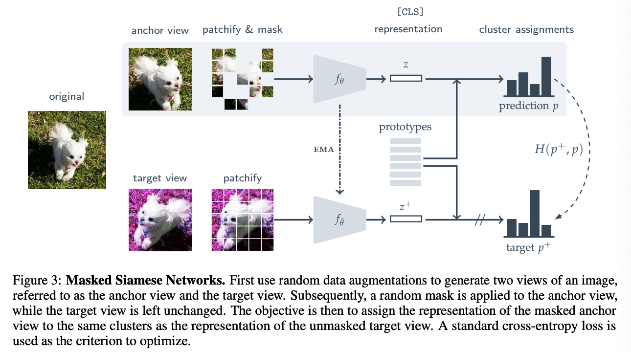
2. Masked Siamese Networks (MSN)
combines invariance-based pre-training with mask denoising
Procedure
- step 1) random data augmentations to generate 2 views of an image
- anchor view & target view
- step 2) random mask is applied to the anchor view
- target view is left unchanged
( like clustering-based SSL approaches … )
\(\rightarrow\) learning occurs by computing a soft-distribution over a set of prototypes for both the anchor & target views
Objective (CE Loss)
-
assign the representation of the masked anchor view,
to the same prototypes as the that of the unmasked target view
(1) Input Views
sample a mini-batch of \(B \geq 1\) images
for each image \(\mathbf{x}_i\) ….
- step 1) apply a random set of data augmentations to generate..
- target view = \(\mathbf{x}_i^{+}\)
- \(M \geq 1\) anchor views = \(\mathbf{x}_{i, 1}, \mathbf{x}_{i, 2}, \ldots, \mathbf{x}_{i, M}\)
(2) Patchify and Mask
step 2) patchify each view ( into \(N \times N\) patches )
step 3) after patchifying the anchor view \(\mathbf{x}_{i, m}\) ….
-
apply the additional step of masking
( by randomly dropping some of the patches )
-
Notation
- \(\hat{\mathbf{x}}_{i, m}\) = sequence of masked anchor
- \(\hat{\mathbf{x}}_i^{+}\) = sequence of unmasked target patches
( because of masking, they can have different length )
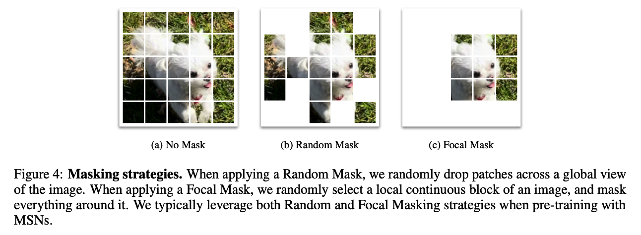
2 strategies for masking the anchor views
- (1) Random Masking
- (2) Focal Masking
(3) Encoder
anchor encoder \(f_\theta(\cdot)\)
-
output : \(z_{i, m} \in \mathbb{R}^d\)
( = representation of patchified (and masked) anchor view \(\hat{\mathbf{x}}_{i, m}\) )
target decoder \(f_{\bar{\theta}}(\cdot)\)
-
output : \(z_i^{+} \in \mathbb{R}^d\)
( = representation of patchified target view \(\hat{\mathbf{x}}_i^{+}\) )
\(\rightarrow\) \(\bar{\theta}\) are updated via an exponential moving average of \(\theta\)
( +Both encoders correspond to the trunk of a ViT )
output of network = representation of [CLS] token
(4) Similarity Metric and Predictions
\(\mathbf{q} \in \mathbb{R}^{K \times d}\) : learnable prototypes
to train encoder …
- compute a distribution based on the similarity between
- (1) prototypes
- (2) each anchor and target view pair
- penalize the encoder for differences between these distributions
For an anchor representation \(z_{i, m}\)…
-
compute a prediction \(p_{i, m} \in \Delta_K\)
( by measuring the cosine similarity to the prototypes matrix \(\mathbf{q} \in \mathbb{R}^{K \times d}\) )
-
predictions \(p_{i, m}\) : \(p_{i, m}:=\operatorname{softmax}\left(\frac{z_{i, m} \cdot \mathbf{q}}{\tau}\right)\)
For an target representation \(z_i^{+}\) ….
-
generate a prediction \(p_i^{+} \in \Delta_K\)
( by measuring the cosine similarity to the prototypes matrix \(\mathbf{q} \in \mathbb{R}^{K \times d}\) )
-
predictions \(p_{i, m}^{+}\) : \(p_{i, m}^{+}:=\operatorname{softmax}\left(\frac{z_{i, m} \cdot \mathbf{q}}{\tau^{+}}\right)\)
\(\rightarrow\) always choose \(\tau^{+}<\tau\) to encourage sharper target predictions
(5) Training Objective
when training encoder…
\(\rightarrow\) penalize when the anchor prediction \(p_{i, m}\) is different from the target prediction \(p_i^{+}\)
( enforce this by using CE-loss \(H\left(p_i^{+}, p_{i, m}\right)\). )
also, incorporate mean entropy maximization (ME-MAX) regularizer
( to encourage the model to utilize the full set of prototypes )
- average prediction across all the anchor views = \(\bar{p}:=\frac{1}{M B} \sum_{i=1}^B \sum_{m=1}^M p_{i, m}\)
- meaning = maximize \(H(\bar{p})\)
overall objective
- parameter : encoder parameters \(\theta\) and prototypes \(q\)
- loss function : \(\frac{1}{M B} \sum_{i=1}^B \sum_{m=1}^M H\left(p_i^{+}, p_{i, m}\right)-\lambda H(\bar{p})\)
( aware ) only compute gradients with respect to the anchor predictions \(p_{i, m}\)
( not the target predictions \(p_i^{+}\) )