LLaVE; Large Language and Vision Embedding Models with Hardness-Weighted Contrastive Learning

LLaVE: Large Language and Vision Embedding Models with Hardness-Weighted Contrastive Learning

Contents

1. Abstract
2. Introduction
3. Preliminary Study
4. Our Framework
   1. Hardness-Weighted CL
   2. Cross-Device Negative Sampling Gathering
5. Experiments
   1. Setup
   2. Main Results
   3. Ablation Study
   4. Zero-shot Video Retrieval
6. Related Work
7. Conclusion

0. Abstract

Universal multimodal embedding models

\(\rightarrow\) Critical role in tasks like ..

• Interleaved image text retrieval
• Multimodal RAG
• Multimodal clustering

[Findings] Existing LMM-based embedding models

• Trained with the “Standard InfoNCE” loss

  \(\rightarrow\) Exhibit a high degree of overlap in similarity distribution btw pos & neg pairs!

  \(\rightarrow\) Challenging to distinguish hard negative pairs effectively!

Proposal: LLaVE

Simple yet effective framework

Dynamically improves the embedding model’s representation learning for negative pairs

\(\rightarrow\) Based on their discriminative difficulty!

Evaluation: MMEB benchmark

• Covers 4 meta-tasks and 36 datasets
• Establishes stronger baselines that achieve SoTA
• Strong scalability and efficiency

Details

• [LLaVE-2B]: Surpasses the previous SOTA 7B model

• [LLaVE-7B]: Achieves a further performance improvement of 6.2 points

• Although LLaVE is trained on image-text data…

  \(\rightarrow\) Generalize to text-video retrieval tasks in a zero-shot manner & Achieve strong performance

1. Introduction

Multimodal embedding models

• Aim to encode inputs from any modality into vector representations
• Facilitate various multimodal tasks
  • Image-text retrieval (Wu et al., 2021; Zhang et al., 2024a)
  • Automatic evaluation (Hessel et al., 2021)
  • Retrieval-augmented generation (RAG) (Zhao et al., 2023)

Pretrained VLMs

(e.g., CLIP (Radford et al., 2021), ALIGN (Jia et al., 2021), and SigLIP (Zhai et al., 2023))

• Provide unified representations for text and images
• Face difficulties when dealing with more complex tasks!
• Adopt a dual-encoder architecture
  • Encodes images and text separately
  • Leading to poor performance in tasks such as interleaved image-text retrieval

LMM-based multimodal embedding models (LMMs)

• (vs. traditional pretrained VLMs)

  • Demonstrate superior multimodal semantic understanding capabilities
  • Also naturally support interleaved text and image inputs.

  \(\rightarrow\) More flexible and efficient in handling multimodal embedding tasks

[Examples of LMMs] Jiang et al. (2024b): Construct the Massive Multimodal Embedding Benchmark (MMEB)

• Encompasses 4 meta-tasks and 36 datasets

• Train multimodal embedding models based on LMMs

• Experiments: By providing suitable task instructions and employing contrastive learning for training…

  \(\rightarrow\) LMM can significantly outperform existing multimodal embedding models and generalize effectively across diverse tasks

Figure 1(a)

When training an LMM as a multimodal embedding model using the standard InfoNCE loss

\(\rightarrow\) Query-target similarity distribution of positive and negative pairs exhibits significant overlap

\(\rightarrow\) Struggles to learn discriminative multimodal representations for positive and hard negative pairs

LLaVE (Large Language and Vision Embedding Models)

Background

• (1) Findings in Figure 1(a)
• (2) Preference learning (Rafailov et al., 2023; Song et al., 2024)

Proposal

• Simple yet effective framework to encourage the model to focus more on HARD negative pairs

• Forcing it to learn more discriminative multimodal representations

• Details

  • Embedding model as a policy model

  • Reward model to assign an adaptive weight to each negative pair

    • Harder pairs \(\rightarrow\) Larger weights
    • Ensures that harder negative pairs play a more significant role in model training

  • Decouple the reward model from the policy model

    \(\rightarrow\) Can not only use different models for hardness estimation but also leverage manually annotated hardness to enhance the representation learning for specific samples.

Cross-device negative sample gathering strategy

• Inspired by SigLIP (Zhai et al., 2023)
• Significantly alleviates the issue of limited negative samples in LMMs caused by excessive memory usage

Evaulation

• Train a series of multimodal embedding models
• Based on advanced open-source LMMs of varying scales
  • LLaVA-OV-0.5B (Li et al., 2024)
  • Aquila-VL-2B (Gu et al., 2024)
  • LLaVA-OV-7B (Li et al., 2024)
• Benchmark: MMEB
  • [LLaVE-0.5B] Achieves comparable results to that of the previous VLM2Vec (phi-3.5V-4B)
  • [LLaVE-2B] Requires only about 17 hours of training on a single machine equipped with 8 A100 GPUs (40GB) to surpass the SoTA model MMRet7B
    • MMRet7B: pretrained on 27 million image-text pairs
  • [LLaVE-7B] Surpassing the previous SOTA model by 6.2 points

2. Preliminary Study

1. Formulation of multimodal embedding task
2. Standard InfoNCE loss
3. Analysis of similarity distributions of positive and negative pairs

(1) CL for LMM-based Multimodal Embedding Models

Following VLM2Vec (Jiang et al., 2024b).. address the challenge of universal retrieval with LMMs

Notation:

• Query-target pair: \((q, t^+)\)
  • Both q and t+ could be an image, text, or interleaved image-text input
  • \(q\) : Equipped with corresponding task instructions
• Objective: Ensure that the Sim(\(q\) , \(t^{+}\)) > Sim(\(q, t^{-}\))

Procedure

• (Given an LLM) Input the query & target separately

• Obtain their representations
  • By extracting the vector representations of the last token in the final layer
• Result: Mini-batch of training data \({(q_1, t_1), ..., (q_N, t_N)}\)

InfoNCE loss

• \(\mathcal{L} = \frac{1}{N} \sum_{i=1}^{N} \log \underbrace{\frac{e^{s_{i,i}/\tau}}{e^{s_{i,i}/\tau} + \sum_{j \neq i}^{N} e^{s_{i,j}/\tau}}}_{\mathcal{L}_i}\).
  • where \(s_{i,j} = \text{Cosine}(\text{LMM}(q_i), \text{LMM}(t_i))\),
  • \(\tau\) is always set to \(0.02\) (following the setting of VLM2Vec)

(2) Analysis

(Base model) Aquila-VL-2B (Gu et al., 2024)

• Builds upon the LLaVA-OneVision architecture
• Perform CL on the MMEB dataset (following the VLM2Vec setup)

Two groups

• [Hard negative] Five pairs with the highest query-target similarities (excluding the positive pairs)
• [Easy negative] Five pairs with the lowest similarities

Details

• Cosine function to calculate the average query-target similarity for the two groups
• Dataset: SUN397 & RefCOCO

Result:

• Distributions of positive and hard negative pairs exhibit significant overlap
• Distributions of positive and easy negative pairs also demonstrate relatively high similarities.

Randomly select one ID dataset & one OOD dataset (from the four meta-tasks in MMEB)

\(\rightarrow\) Evaluate the model’s average query-to-target similarity on positive, hard negative, and easy negative pairs, respectively.

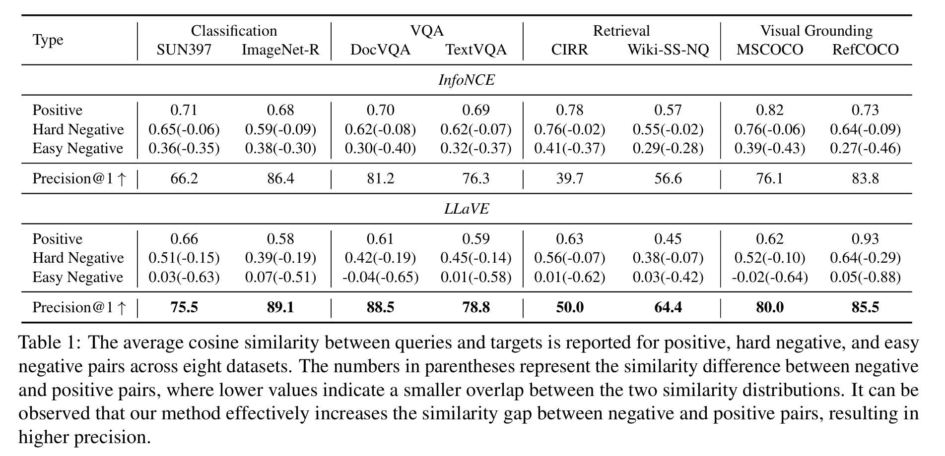
[Table 1]

• Similarity difference between positive vs. negative pairs

• Similarity (trained with InfoNCE loss): Relatively “small” (no more than 0.09)

  \(\rightarrow\) Low precision

  • Smaller the similarity difference, the lower the final precision tends to be

\(\rightarrow\)

Validates the necessity of enhancing learning on hard negative pairs during training!!

\(\rightarrow\) Motivation to explore a simple and effective approach to strengthen the model’s learning of negative pairs with varying difficulty levels

3. Our Framework

• (1) Illustrate the inherent consistency between preference learning & contrastive learning

• (2) Propose a simple yet effective framework

  \(\rightarrow\) Mainly involves hardness-weighted CL & cross-device negative sample gathering

(1) Hardness-Weighted CL

Preference learning & contrastive learning

\(\rightarrow\) Share a fundamental goal

= Modeling relationships between pairs, based on relative preference or similarity of the target within the pairs

a) Preference learning

Involves a reward model & policy model

• (1) Reward model: Scores the outputs of the policy model
• (2) Policy model: Updates its parameters using the feedback from the reward model to produce higher-reward outputs

Bradley-Terry (BT) model (Bradley and Terry, 1952)

• Captures pairwise relationships through probabilistic comparisons

• To directly optimize the embedding model (i.e. the policy model)

  \(\rightarrow\) Follow Song et al. (2024) to consider the embedding model as both the (1) reward model and (2) policy model

Notation

• Query \(q_1\)
• Two targets \(t_1\) and \(t_2\),

BT model: Defines the training objective of preferring \(t_1\) over \(t_2\) as..

• [Eq 2] \(\mathcal{L}_1 = -\log \frac{e^{r_{\pi}(q_1,t_1)}}{e^{r_{\pi}(q_1,t_1)} + e^{r_{\pi}(q_1,t_2)}}\),
  • \(r_{\pi}(\cdot)\) : Function of reward/policy model

One-to-\(N\) contrast setting (Song2024)

• Extension of the BT model

  (= Essentially consistent with the InfoNCE loss)

• [Eq 2 -> 3] \(\mathcal{L}_i = -\log \frac{e^{r_{\pi}(q_i,t_i)}}{e^{r_{\pi}(q_i,t_i)} + \sum_{j \neq i}^{N} e^{r_{\pi}(q_i,t_j)}}\)

  • where \(r_{\pi}(q_i, t_j) = s_{i,j}/\tau\), \(s_{i,j}\)

(Proposed) Hardness-weighted CL

• Assigns weight according to the learning difficulty of the negative pair

• Higher weights = Greater difficulty

  \(\rightarrow\) Incur heavier penalties

  \(\rightarrow\) Encouraging the model to learn more from challenging negative pairs

\(\mathcal{L}_i = -\log \frac{e^{r_{\pi}(q_i,t_i)}}{e^{r_{\pi}(q_i,t_i)} + \sum_{j \neq i}^{N} w_{ij} \cdot e^{r_{\pi}(q_i,t_j)}}\).

• \(w_{ij}\) : Weight of learning difficulty

[Figure 2] To estimate the learning difficulty of pairs …

• Introduce a reward model \(r_{\theta}\)
• Set \(w_{ij} = e^{r_{\theta}(q_i,t_j)}\).

• Policy model: Adjusts its learning of different negative pairs based on the “feedback” from the reward model

• LLaVE: Set the reward model \(r_{\theta}\) == policy model \(r_{\pi}\)
  • Achieve higher training efficiency and simpler implementation
  • w/o backpropagating gradients, i.e. \(r_{\theta}(q_i,t_j) = \alpha \cdot \text{sg}(s_{ij})\)

Loss function of LLaVE \(\mathcal{L}_i\):

• \(\mathcal{L}_i = - \log \frac{e^{r_{\pi}(q_i,t_i)}}{e^{r_{\pi}(q_i,t_i)} + \sum_{j \neq i}^{N} e^{\left(r_{\pi}(q_i,t_j) + r_{\theta}(q_i,t_j)\right)}}\).

Gradients with respect to the \(r_{\pi}(q_i, t_j)\) (\(j \neq i\))

• \(\frac{\partial \mathcal{L}_i}{\partial r_{\pi}(q_i, t_j)} = e^{r_{\theta}(q_i,t_j)} \cdot \frac{e^{r_{\pi}(q_i,t_j)}}{Z_i}\).
• \(Z_i = e^{r_{\pi}(q_i,t_i)} + \sum_{j \neq i}^{N} e^{\left(r_{\pi}(q_i,t_j) + r_{\theta}(q_i,t_j)\right)}\).

\(\rightarrow\) Gradients of the negative pairs are proportional to the product \(r_{\theta}(q_i,t_j)\)

\(\rightarrow\) Implies that the “greater the learning difficulty” of a negative pair, “the more significant” its role in the gradient update.

(2) Cross-Device Negative Sample Gathering

# of negative pairs in CL

\(\rightarrow\) Important effect on model training

LMM-based embedding models

• Face the challenge of high memory consumption

  \(\rightarrow\) Making it diff icult to use a large batch size directly!

• Solution: Cross-device negative sample gathering strategy

  • Inspired by OpenCLIP (Cherti et al., 2023) and SigLIP (Zhai et al., 2023),
  • Increases the number of negative pairs by a factor of the device number \(K\)

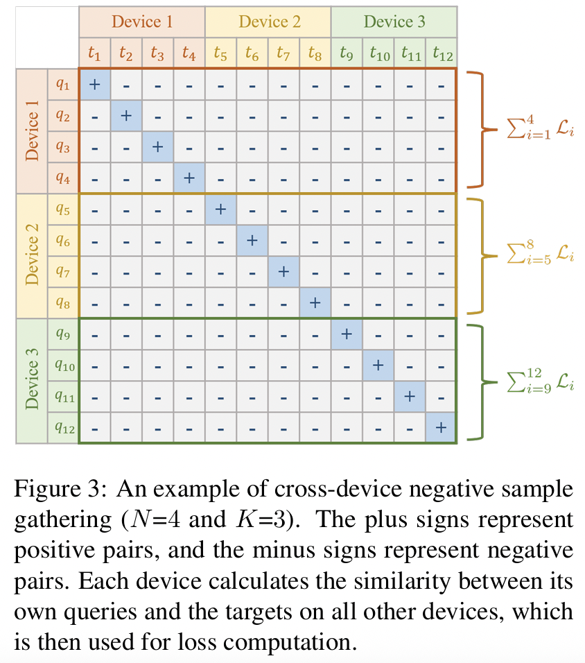
• Expand the number of negative pairs on each device
• By gathering samples from other devices

w/o & w/ cross-device negative sampling gathering

• [w/o] \(\mathcal{L}_i = - \log \frac{e^{r_{\pi}(q_i,t_i)}}{e^{r_{\pi}(q_i,t_i)} + \sum_{j \neq i}^{N} e^{\left(r_{\pi}(q_i,t_j) + r_{\theta}(q_i,t_j)\right)}}\).
• [w/] \(\mathcal{L}_i = -\log \frac{e^{r_{\pi}(q_i,t_i)}}{e^{r_{\pi}(q_i,t_i)} + \sum_{j \neq i}^{N \cdot K} e^{\left(r_{\pi}(q_i,t_j) + r_{\theta}(q_i,t_j)\right)}}\).

\(\rightarrow\) Effectively increase the number of negative pairs w/o significantly increasing memory consumption

4. Experiments

(1) Setup

a) Datasets and Metrics

(Follow VLM2Vec (Jiang et al., 2024b))

[Train] 20 in-distribution datasets from MMEB

• Encompass four meta-tasks
  • classification, VQA, multimodal retrieval, and visual grounding
• Total of 662K training pairs.

[Eval] 20 in-distribution and 16 out-of-distribution test sets from MMEB

[Metric] Precision@1 on each dataset

• Measures the proportion of top-ranked candidates that are positive samples.

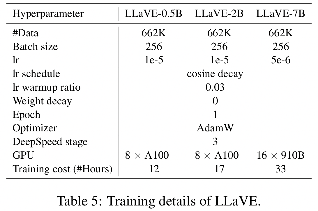
b) Implementation Details

Three scales: 0.5B, 2B, 7B

• [0.5B] LLaVA-OV-0.5B (Li et al., 2024)
• [2.0B] AquilaVL-2B (Gu et al., 2024)
• [7.0B] LLaVA-OV-7B (Li et al., 2024)

Hyperparameters

• Batch size = 256
• Weighting hyperparameter \(\alpha\) = 9
• Total length limit = 4096
• Learning rate
  • [0.5B, 2B] 1e-5
  • [7B] 5e-6
• Epoch = 1 (with DeepSpeed ZeRO-3 strategy)

Higher Anyres technique (Li et al., 2024):

• To support high-resolution images

  (Maximum image resolution to 672 × 672)

Freeze & Train

• [Freeze] Vision encoder
• [Train] Connector & LLM

Resources

• [0.5B, 2B] 8A100 GPUs (40GB) for 12 and 17 hours
• [7B] 16 Ascend 910B GPUs (64GB) for 33 hours

c) Baselines

(Following VLM2Vec)

• CLIP (Radford et al., 2021)
• OpenCLIP (Cherti et al., 2023)
• BLIP2 (Li et al., 2023a)
• SigLIP (Zhai et al., 2023)
• UniIR (Wei et al., 2024)
• E5-V (Jiang et al., 2024a)

• Magiclens (Zhang et al., 2024b)

• VLM2Vec (Jiang et al., 2024b)
• MMRet-MLLM(Zhou et al., 2024)
  • Enhances downstream task performance through pretraining on a self-built retrieval dataset (consisting of 26M pairs)

(For fair comparison) Also compare the VLM2Vec trained using the same base LMM

• VLM2Vec (LLaVA-OV-0.5B)
• VLM2Vec (Aquila-VL-2B)
• VLM2Vec (LLaVA-OV-7B)

(2) Main Results

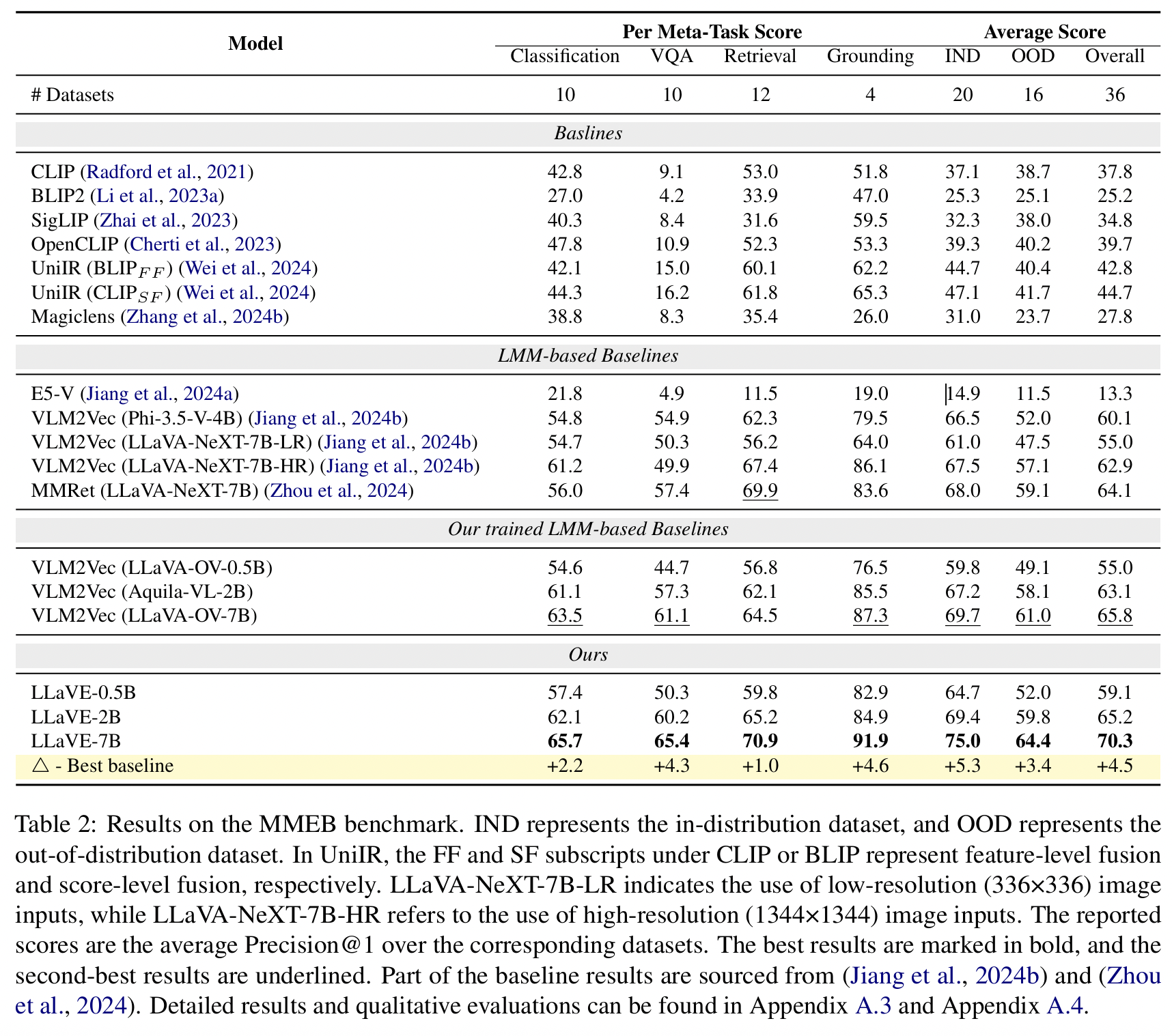
LLaVE series (LLaVE-0.5B, LLaVE2B, LLaVE-7B) vs. Existing baseline models

a) Baselines

a) VLM2Vec (LLaVA-OV-7B)

• Achieves the highest overall average score of 65.8
• Surpass current SoTA (MMRet: 64.1)

\(\rightarrow\) Findings 1) A more powerful foundational LMM can lead to better performance

b) MMRet

• Excels in retrieval tasks with a score of 69.9

  (\(\because\) Pretraining on its self-constructed 26M image-text retrieval dataset)

c) VLM2Vec (LLaVA-NeXT-7B-HR)

• Exhibits superior performance in grounding tasks

  (\(\because\) Due to its higher input image resolution)

b) LLaVE series

Demonstrates consistent improvements over the best baseline across all metrics

[Overall score]

• MMRet: 64.1
• VLM2Vec (LLaVA-OV-7B): 65.8
• LLaVE-7B: 70.3

Performance of LLaVE-7B

• Grounding: 91.9
• VQA: 65.4
• Classification: 65.7

Scalability: Performance scales consistently with model size!

• Performance of LLaVE-0.5B is already comparable to VLM2Vec(Phi-3.5-V-4B)

(3) Ablation Study

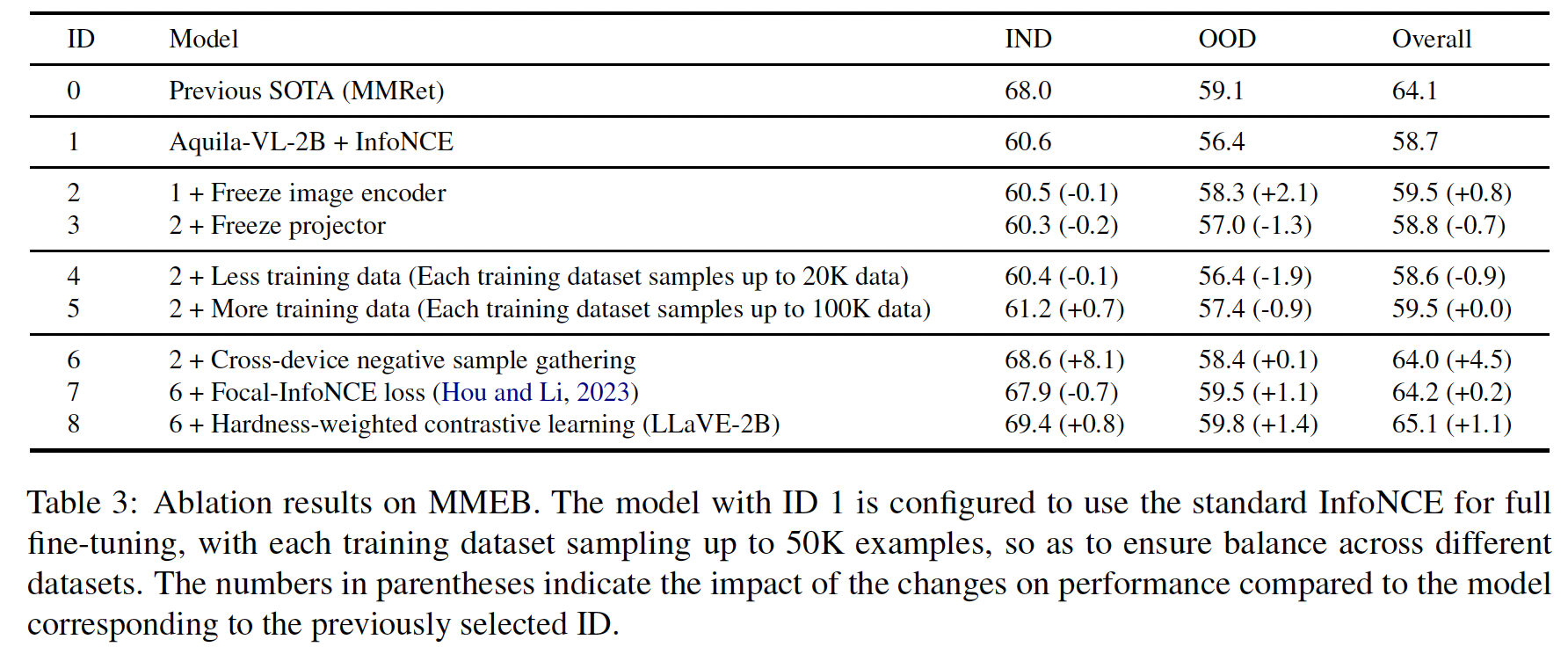
• (1) Freezing the image encoder helps generalize to OOD datasets
• (2) When the dataset is sufficient, balanced distribution of various data is more important than simply having more data
• (3) # of negatives is crucial for training LMM-based embedding models
• (4) Hardness-weighted CL can further enhance the performance of powerful models on both ID & OOD

(4) Zero-shot Video Retrieval

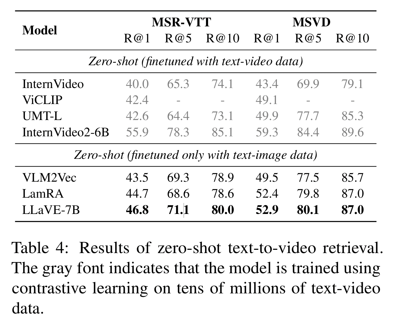
Text-video retrieval datasets: MSR-VTT and MSVD

Two types of comparative models

• (1) Models trained on tens of millions of video-text data
  • e.g., InternVideo, ViCLIP, UMT-L, InternVideo2-6B
• (2) Zero-shot, trained only on text-image data using CL & Directly evaluated on text-video data
  • e.g., VLM2Vec (LLaVA-OV-7B), LamRA (based on Qwen2-VL-7B)
    • LamRA consists of two 7B models: LamRA-Ret and LamRA-Rank
      • LamRA-Ret: Retrieves the top-\(K\) candidates
      • LamRA-Rank: Re-ranks these retrieved candidates.

To enable video embedding, we ..

• Set the maximum number of sampled frames to 32
• Expand the total input length of the model to 8192
• Reduce the visual features of the video by 4 times through bilinear interpolation

Results

• (Compared to LamRA) LLaVE-7B requires only a single model & shows consistent improvements across all metrics

• Although LLaVE-7B does not utilize text-video data for CL, its performance still surpasses most video retrieval models

  • Except for InternVideo2-6B, which are trained on tens of millions of video-text pairs.

  \(\rightarrow\) Demonstrate that LLaVE-7B has strong potential for transferring to other embedding tasks!

5. Related Work

(1) Multimodal Embeddings

Aim to integrate the information from “multiple” modalities into a “shared” representation space

\(\rightarrow\) Enables seamless understanding across modalities

[Early research]

Focuses on leveraging dual-stream architectures

= Separately encode texts and images

• e.g., CLIP, ALIGN, BLIP, SigLIP: Adopt “dual-encoder” frameworks

[Recent works]

• To learn the more universal multimodal representations

• UniIR: Two fusion mechanisms

  • Combine the visual and textual representations generated by the dual-encoder model

  \(\rightarrow\) Still face challenges in handling tasks in ..

  • Interleaved image-text retrieval
  • Instruction-following multimodal retrieval

(2) LMM-based Multimodal Embeddings

E5-V & VLM2Vec

• Transform “LMM” into “multimodal embedding models” through CL
• Fully leverage LMM’s powerful multimodal understanding capability and its inherent advantage in handling interleaved text-image input

Few concurrent studies

• Explored the application of LMMs in multimodal embeddings
• LamRA
  • Adopts the retrieval model to select the top-\(K\) candidates
  • Then scored by the reranking models.
  • Scores from the retrieval and reranking models are combined using a weighted sum to produce the final score for retrieval.
• MMRet
  • Creates a large-scale multimodal instruction retrieval dataset called MegaPairs
  • By pretraining on this dataset, MMRet achieves SOTA results on MMEB.

(3) CL

Negative samples play a crucial role in CL

• SimCLR: Incorporating more negative samples can enhance the performance of CL
• Awasthi2022: Explore the impact of the number of negative samples from both theoretical and empirical perspectives
• Cai2020: Demonstrate that hard negative samples are both necessary and sufficient to learn more discriminative representation
• Robinson2021: Propose a hard negative sampling strategy
  • where the user can control the hardness
• Focal-InfoNCE (Hou2023): Weighs both positive and negative pairs based on their query-target similarities
  • Uses a fixed threshold to determine the hardness of negative pairs
  • Increasing the weight if the similarity exceeds the threshold
  • Decreasing it otherwise.

(Proposed) Hardness-weighted CL

• Introduces a reward model to dynamically estimate the hardness of negative pairs

• Applies weighting only to the negative pairs based on the estimated hardness.

  (Notably, the reward model can be decoupled from the policy model)

6. Conclusion

• Findings: LMM-based embedding models trained with the standard InfoNCE loss face significant challenges in handling hard negative pairs

• Proposal:

  • (1) Hardness-weighted CL
  • (2) Cross-device negative sample gathering strategy

  \(\rightarrow\) To enhance the model’s learning of negative pairs with varying difficulty levels

  \(\rightarrow\) Significantly improves the model’s capacity to distinguish between positive and negative pairs.

• Limitations: Trained only on embedding datasets that contain arbitrary combinations of text and image modalities

  • Significant room for improvement

  \(\rightarrow\) Constructing a multimodal embedding benchmark that incorporates the video modality will be a crucial direction!