
DCdetector: Dual Attention Contrastive Representation Learning for TS Anomaly Detection (KDD 2023)
https://arxiv.org/pdf/2306.10347.pdf
Contents
- Abstract
- Introduction
- Methodology
- Overall Architecture
- Dual Attention Contrastive Structure
- Representation Discrepancy
- Anomaly Criterion
0. Abstract
Challenge of TS anomaly detection
- learn a representation map that enables effective discrimination of anomalies.
Categories of methods
- Reconstruction-based methods
- Contrastive learning
DCdetector
- a multi-scale dual attention contrastive representation learning model
- utilizes a novel dual attention asymmetric design to create the permutated environment
- learn a permutation invariant representation with superior discrimination abilities
1. Introduction
Challenges in TS-AD
- (1) Determining what the anomalies will be like.
- (2) Anomalies are rare
- hard to get labels
- most supervised or semi-supervised methods fail to work given limited labeled training data.
- (3) Should consider temporal, multidimensional, and non-stationary features for TS
TS anomaly detection methods
( ex. statistical, classic machine learning, and deep learning based methods )
- Supervised and Semi-supervised methods
- can not handle the challenge of limited labeled data
- Unsupervised methods
- without strict requirements on labeled data
- ex) one class classification-based, probabilistic based, distance-based, forecasting-based, reconstruction-based approaches
Examples
- Reconstruction-based methods
- pros) developing rapidly due to its power in handling complex data by combining it with different machine learning models and its interpretability that the instances behave unusually abnormally.
- cons) challenging to learn a well-reconstructed model for normal data without being obstructed by anomalies.
- Contrastive Learning
- outstanding performance in downstream tasks in the computer vision
- effectiveness of contrastive representative learning still needs to be explored in the TS-AD
DCdetector
( Dual attention Contrastive representation learning anomaly detector )
-
handle the challenges in TS AD
-
key idea : normal TS points share the latent pattern
( = normal points have strong correlations with other points <-> anomalies do not )
- Learning consistent representations :
- hard for anomalies
- easy for normal points
- Motivation : if normal and abnormal points’ representations are distinguishable, we can detect anomalies without a highly qualified reconstruction model
Details
- contrastive structure with two branches & dual attention
- two branches share weights
- representation difference between normal and abnormal data is enlarged
- patching-based attention networks: to capture the temporal dependency
- multi-scale design: to reduce information loss during patching
- channel independence design for MTS
- does not require prior knowledge about anomalies
2. Methodology
MTS of length \(\mathrm{T}\) : \(X=\left(x_1, x_2, \ldots, x_T\right)\)
- where \(x_t \in \mathbb{R}^d\)
Task:
- given input TS \(\mathcal{X}\),
-
for another unknown test sequence \(\mathcal{X}_{\text {test }}\) of length \(T^{\prime}\)
- we want to predict \(\mathcal{Y}_{\text {test }}=\left(y_1, y_2, \ldots, y_{T^{\prime}}\right)\).
- \(y_t \in\{0,1\}\) : 1 = anomaly & 0 = normal
Inductive bias ( as Anomaly Transformer explored )
- anomalies have less connection with the whole TS than their adjacent points
- Anomaly Transformer: detects anomalies by association discrepancy between ..
- (1) a learned Gaussian kernel
- (2) attention weight distribution.
- DCdetector
- via a dual-attention self-supervised contrastive-type structure.
Comparison
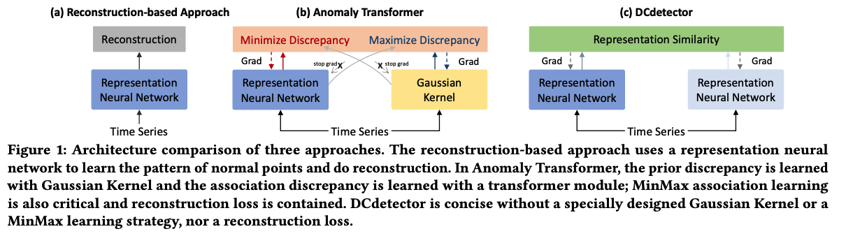
- Reconstruction-based approach
- Anomaly Transformer
- observation that it is difficult to build nontrivial associations from abnormal points to the whole series.
- discrepancies
- prior discrepancy : learned with Gaussian Kernel
- association discrepancy : learned with a transformer module
- MinMax association learning & Reconstruction loss
- DCdetector
- concise ( does not need a specially designed Gaussian Kernel, a MinMax learning strategy, or a reconstruction loss )
- mainly leverages the designed CL-based dual-branch attention for discrepancy learning of anomalies in different views
(1) Overall Architecture
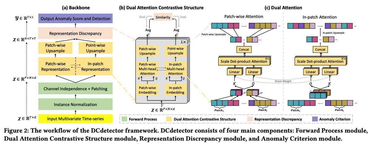
4 main components
- Forward Process module
- Dual Attention Contrastive Structure module
- Representation Discrepancy module
- Anomaly Criterion module.
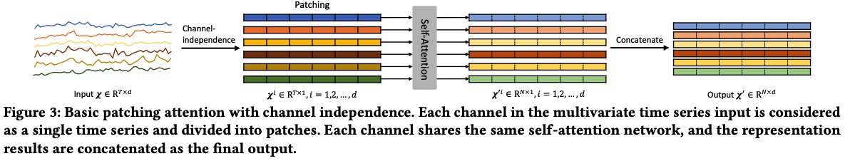
a) Forward Process module
( channel-independent )
- a-1) instance normalization
- a-2) patching
b) Dual Attention Contrastive Structure module
- each channel shares the same self-attention network
- representation results are concatenated as the final output \(\left(X^{\prime} \in \mathbb{R}^{N \times d}\right)\).
- Dual Attention Contrastive Structure module
- learns the representation of inputs in different views.
c) Representation Discrepancy module
Key Insight
- normal points: share the same latent pattern even in different views (a strong correlation is not easy to be destroyed).
- anomalies: rare & do not have explicit patterns
\(\rightarrow\) difference will be slight for normal points representations in different views and large for anomalies.
d) Anomaly Criterion module.
-
calculate anomaly scores based on the discrepancy between the two representations
-
use a prior threshold for AD
(2) Dual Attention Contrastive Structure
TS from different views: takes ..
- (1) patch-wise representations
- (2) in-patch representations
Does not construct pairs like the typical contrastive methods
- similar to the contrastive methods only using positive samples
a) Dual Attention
Input time series \(\mathcal{X} \in \mathbb{R}^{T \times d}\) are patched as \(\mathcal{X} \in \mathbb{R}^{P \times N \times d}\)
- \(P\) : patch size
- \(N\) : number of patches
Fuse the channel information with the batch dimension ( \(\because\) channel independence )
\(\rightarrow\) becomes \(\mathcal{X} \in \mathbb{R}^{P \times N}\).
[ Patch-wise representation ]
- single patch is considered as a unit
- embedded operation will be applied in the patch_size \((P)\) dimension
- capture dependencies among patches ( = patch-wise attention )
- embedding shape : \(X_{\mathcal{N}} \in \mathbb{R}^{N \times d_{\text {model }}}\).
- apply multi-head attention to \(X_{\mathcal{N}}\)
[ In-patch representation ]
- dependencies of points in the same patch
- embedded operation will be applied in the number of patches \((N)\) dimension
Note that the \(W_{Q_i}, W_{\mathcal{K}_i}\) are shared weights within the in-patch & patch-wise attention
b) Up-sampling and Multi-scale Design
Patch-wise attention
- ignores the relevance among points in a patch
In-patch attention
- ignores the relevance among patches.
To compare these two representations …. need upsampling!
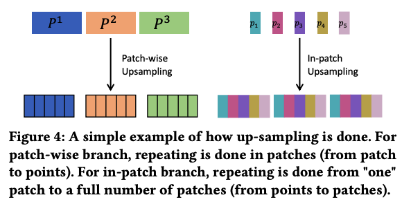
Multi-scale design:
= final representation concatenates results in different scales (i.e., patch sizes)
- final patch-wise representation: \(\mathcal{N}\)
- \(\mathcal{N}=\sum_{\text {Patch list }} \operatorname{Upsampling}\left(\text { Attn }_{\mathcal{N}}\right)\),
- Final in-patch representation: \(\mathcal{P}\)
- \(\mathcal{P}=\sum_{\text {Patch list }} \text { Upsampling }\left(\text { Attn }_{\mathcal{P}}\right)\).
c) Contrastive Structure
Patch-wise sample representation
- learns a weighted combination between sample points in the same position from each patch
In-patch sample representation
- learns a weighted combination between points within the same patch.
\(\rightarrow\) Treat these two representations as “permutated multi-view representations”
(3) Representation Discrepancy
Kullback-Leibler divergence (KL divergence)
- to measure the similarity of such two representations
Loss function definition
( no reconstruction part is used )
\(\mathcal{L}\{\mathcal{P}, \mathcal{N} ; X\}=\frac{1}{2} \mathcal{D}(\mathcal{P}, \operatorname{Stopgrad}(\mathcal{N}))+\frac{1}{2} \mathcal{D}(\mathcal{N}, \operatorname{Stopgrad}(\mathcal{P}))\).
- Stop-gradient : to train 2 branches asynchronously
(4) Anomaly Criterion
Final anomaly score of \(\mathcal{X} \in \mathbb{R}^{T \times d}\) :
- \(\text { AnomalyScore }(X)=\frac{1}{2} \mathcal{D}(\mathcal{P}, \mathcal{N})+\frac{1}{2} \mathcal{D}(\mathcal{N}, \mathcal{P}) \text {. }\).
\(y_i= \begin{cases}1: \text { anomaly } & \text { AnomalyScore }\left(X_i\right) \geq \delta \\ 0: \text { normal } & \text { AnomalyScore }\left(X_i\right)<\delta\end{cases}\).