C-Mamba: Channel Correlation Enhanced State Space Models for Multivariate Time Series Forecasting
Contents
- Abstract
- Introduction
- Preliminray
- MTS forecasting
- Mamba
- Methodology
- Channel Mixup
- C-Mamba Block
- Experiments
0. Abstract
Limitations of previous models
- Linear: limit in capacities
- Attention: quadratic complexity
- CNN: restricted receptive field
CI strategy: ignoring their correlations!!
CD strategy: considering inter-channel relationships
-
Via self-attention mechanism, linear combination, or convolution …
\(\rightarrow\) high computational costs
C-Mamba
-
(1) SSM that captures (2) cross-channel dependencies ,
while maintaining (3) linear complexity (4)without losing the global receptive field
-
Components
- (1) Channel mixup
- two channels are mixed to enhance the training sets
- (2) Channel attention enhanced patch-wise Mamba encoder
- leverages the ability of the SSM
- capture cross-time dependencies and models correlations between channels by mining their weight relationships.
- (1) Channel mixup
1. Introduction
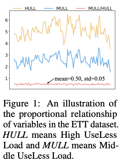
Cross-channel dependencies are also vital for MTSF!
Ex) two variables over time in the ETT
Observations:
-
(1) Two variables exhibit strong temporal characteristics similarity
-
(2) Show a strong proportional relationship
-
MULL (Middle UseLess Load) = 1/2 x HULL (High UseLess Load)
\(\rightarrow\) Necessity of modeling cross-channel dependencies from proportional relationships
-
C-Mamba
-
To better capture cross-time and cross-channel dependencies
-
Channel enhanced SSM
-
Problem & Solution [1]
-
Problem) Oversmoothing caused by the CD
-
Solution) Channel mixup strategy
-
inspired by mixup data augmentation
-
fuses two channels via a linear combination for training
( = generate virtual channel )
-
Generate virtual channel integrate characteristics from different channels while retaining their shared cross-time dependencies, which is expected to improve the generalizability of models.
-
-
-
Problem & Solution [2]
- Problem) Capturing both cross-time and cross-channel dependencies
- Solution) Channel attention enhanced patch-wise Mamba encoder
- a) Cross-time dependencies: via Mamba ( + Patching )
- Patch-wise Mamba module
- b) Cross-channel dependencies: via channel attention
- Lightweight mechanism that considers various relationships between channels
- (1) weighted summation relationships & (2) proportional relationships
- Lightweight mechanism that considers various relationships between channels
- a) Cross-time dependencies: via Mamba ( + Patching )
2. Preliminary
(1) MTS forecasting
Notation
- \(\mathbf{X}=\left\{\mathbf{x}_1, \ldots, \mathbf{x}_L\right\} \in \mathbb{R}^{L \times V}\) ,
- \(\mathbf{X}_{t,:}\) : value of all channels at time step \(t\),
- \(\mathbf{X}_{:, v}\) as the entire sequence of the channel indexed by \(v\)
- \(\mathbf{Y}=\left\{\mathbf{x}_{L+1}, \ldots, \mathbf{x}_{L+T}\right\} \in \mathbb{R}^{T \times V}\).
(2) Mamba
Notation
- Input \(\mathbf{x}(t) \in \mathbb{R}\),
- Output \(\mathbf{y}(t) \in \mathbb{R}\),
- Hidden state \(\mathbf{h}(t) \in \mathbb{R}^N\)
\(\begin{aligned} \mathbf{h}^{\prime}(t) & =\mathbf{A h}(t)+\mathbf{B x}(t), \\ \mathbf{y}(t) & =\mathbf{C h}(t), \end{aligned}\).
- \(\mathbf{A} \in \mathbb{R}^{N \times N}\) : state transition matrix,
- \(\mathbf{B} \in \mathbb{R}^{N \times 1}\) and \(\mathbf{C} \in \mathbb{R}^{1 \times N}\) : projection matrices
Multivariate TS
- \(\mathbf{x}(t) \in \mathbb{R}^V\) and \(\mathbf{y}(t) \in \mathbb{R}^V\),
- \(\mathbf{A} \in \mathbb{R}^{V \times N \times N}, \mathbf{B} \in \mathbb{R}^{V \times N}\), \(\mathbf{C} \in \mathbb{R}^{V \times N}\).
- \(\mathbf{A}\) can be compressed to \(V \times N\)
Discreticize
\(\begin{aligned} \overline{\mathbf{A}} & =\exp (\Delta \mathbf{A}) \\ \overline{\mathbf{B}} & =(\Delta \mathbf{A})^{-1}(\exp (\Delta \mathbf{A})-\mathbf{I}) \Delta \mathbf{B} \\ \mathbf{h}_t & =\overline{\mathbf{A}} \mathbf{h}_{t-1}+\overline{\mathbf{B}} \mathbf{x}_t \\ \mathbf{y}_t & =\mathbf{C h}_t \end{aligned}\).
- where \(\Delta \in \mathbb{R}^V\) is the sampling time interval
Global convolution
\(\begin{aligned} & \overline{\mathbf{K}}=\left(\mathbf{C} \overline{\mathbf{B}}, \mathbf{C A B}, \ldots, \mathbf{C} \overline{\mathbf{A}}^{L-1} \overline{\mathbf{B}}\right) \\ & \mathbf{Y}=\mathbf{X} * \overline{\mathbf{K}}, \end{aligned}\).
- where \(L\) is the length of the sequence.
Selective scan mechanism
Selective scan strategy ( Data-dependent mechanism )
- \(\mathbf{B} \in \mathbb{R}^{L \times V \times N}, \mathbf{C} \in \mathbb{R}^{L \times V \times N}\),
- \(\Delta \in \mathbb{R}^{L \times V}\) : derived from the input \(\mathbf{X} \in \mathbb{R}^{L \times V}\).
3. Methodology
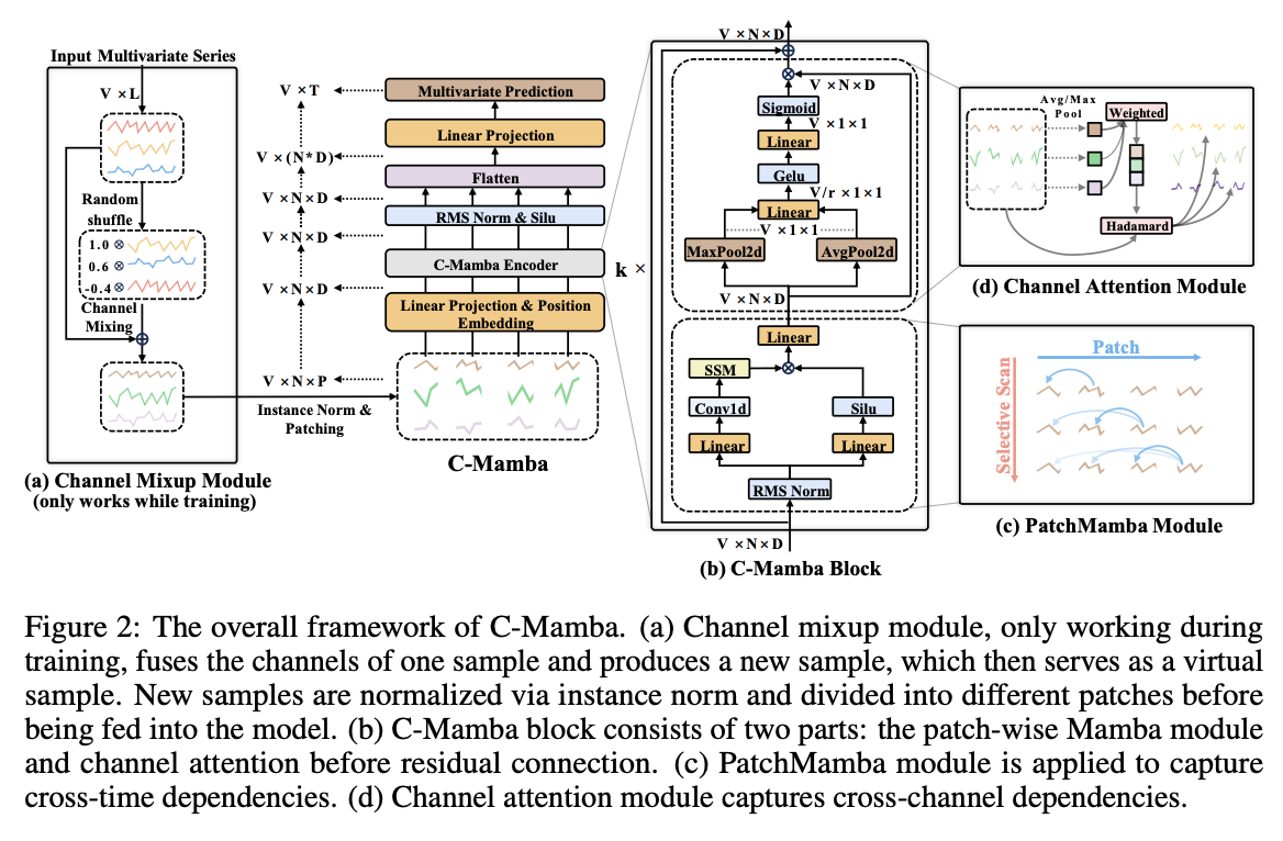
Before training
- Channel mixup module: Mixes MTS in channel dim
Model
- C-Mamba block
- Vanilla Mamba module
- Channel attention module
- Exploits both cross-time and cross-channel dependencies.
- Patch-wise sequences
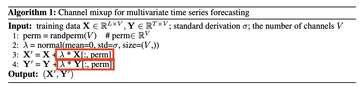
(1) Channel Mixup
Mixup
\(\begin{aligned} & \tilde{x}=\lambda x_i+(1-\lambda) x_j \\ & \tilde{y}=\lambda y_i+(1-\lambda) y_j \end{aligned}\).
- where \((\tilde{x}, \tilde{y})\) is the synthesized virtual sample, and \(\lambda \in[0,1]\).
Channel Mixup
\(\begin{aligned} & \mathbf{X}^{\prime}=\mathbf{X}_{:, i}+\lambda \mathbf{X}_{:, j}, i, j=0, \ldots, V-1 \\ & \mathbf{Y}^{\prime}=\mathbf{Y}_{:, i}+\lambda \mathbf{Y}_{:, j}, i, j=0, \ldots, V-1 \end{aligned}\).
- where \(\mathbf{X}^{\prime} \in \mathbb{R}^{L \times 1}\) and \(\mathbf{Y}^{\prime} \in \mathbb{R}^{T \times 1}\) are hybrid channels
- where randperm \((V)\) generates a randomly arranged array of \(0 \sim V-1\)
- \(\lambda \sim N\left(0, \sigma^2\right)\) is the linear combination coefficient
Normal distribution with a mean of 0
\(\rightarrow\) Ensuring that the overall characteristics of each channel remain unchanged.
(2) C-Mamba Block
Consists of two key components:
- (1) Patch-wise Mamba module
- (2) Channel attention module
\(\rightarrow\) Capture cross-time and cross-channel dependencies respectively!
a) PatchMamba
Patching
- Each univariate TS \(\mathbf{X}_{: v} \in \mathbb{R}^L\),
- \(\hat{\mathbf{X}}_{: v}=\operatorname{Patching}\left(\mathbf{X}_{: v}\right) \in \mathbb{R}^{N \times P}\).
b) Channel Attention
Structure of the channel attention module.
Notation:
-
\(\mathbf{H}_l \in \mathbb{R}^{V \times N \times D}\): Embedding after the \(l^{t h}\) PatchMamba module
-
\(\operatorname{Att}_l=\operatorname{sigmoid}\left(\operatorname{MLP}\left(\operatorname{MaxPool}\left(\mathbf{H}_l\right)\right)+\operatorname{MLP}\left(\operatorname{AvgPool}\left(\mathbf{H}_l\right)\right)\right)\).
- AvgPool and MaxPool : applied to the last two dimensions
-
\(\operatorname{Att}_l=\operatorname{sigmoid}\left(\mathbf{W}_1\left(\operatorname{Gelu}\left(\mathbf{W}_0 \mathbf{F}_{\text {max }}^l\right)\right)+\mathbf{W}_1\left(\operatorname{Gelu}\left(\mathbf{W}_0 \mathbf{F}_{\text {avg }}^l\right)\right)\right)\).
-
\(\mathbf{F}_{\text {max }}^l \in \mathbb{R}^{V \times 1 \times 1}\) and \(\mathbf{F}_{\text {avg }}^l \in \mathbb{R}^{V \times 1 \times 1}\) ,
-
\(\mathbf{W}_0 \in \mathbb{R}^{V / r \times V}\) and \(\mathbf{W}_1 \in \mathbb{R}^{V \times V / r}\),
-
\(r\): controlling the parameter complexity, denotes the reduction ratio.
( = Essential for time series with hundreds of channels, tune it in \(\{2,4,8\}\). )
-
-
-
\(\operatorname{Att}_l \in \mathbb{R}^{V \times 1 \times 1}\):
\(\mathbf{C A}_l=\operatorname{Att}_l \odot \mathbf{H}_l .\) : output of the channel attention module
c) Overall Pipeline
(Instance normalization to mitigate the distribution shifts)
-
\(\mathbf{X}^{\prime}, \mathbf{Y}^{\prime}=\operatorname{Mixup}(\mathbf{X}, \mathbf{Y})\).
-
\(\mathbf{X}_{\text {norm }}^{\prime}=\operatorname{InstanceNorm}\left(\mathbf{X}^{\prime}\right)\).
-
\(\hat{\mathbf{X}} =\operatorname{Patching}\left(\mathbf{X}_{\text {norm }}^{\prime}\right)\).
-
\(\mathbf{Z}_0 =\hat{\mathbf{X}} \mathbf{W}_p+\mathbf{W}_{\text {pos }}\).
-
learnable position encoding \(\mathbf{W}_{\text {pos }}\).
-
where \(\hat{\mathbf{X}} \in \mathbb{R}^{V \times N \times P}, \mathbf{W}_p \in \mathbb{R}^{P \times D}, \mathbf{W}_{\text {pos }} \in \mathbb{R}^{N \times D}\), and \(\mathbf{Z}_0 \in \mathbb{R}^{V \times N \times D}\)
-
[C-mamba encoder .. k blocks]
-
\(\begin{aligned} \mathbf{H}_l & =\operatorname{PatchMamba}\left(\mathbf{Z}_{l-1}\right), \\ \mathbf{Z}_l & =\operatorname{Att}_l\left(\mathbf{H}_l\right) \odot \mathbf{H}_l+\mathbf{Z}_{l-1} \end{aligned}\).
-
\(\hat{\mathbf{Y}}_p=\operatorname{Flatten}\left(\operatorname{Silu}\left(\operatorname{RMS}\left(\mathbf{Z}_k\right)\right)\right) \mathbf{W}_{p r o j}\).
- linear projection layer: \(\mathbf{W}_{p r o j} \in \mathbf{R}^{(N * D) \times T}\)
- \(\hat{\mathbf{Y}}_p \in \mathbb{R}^{V \times T}\).
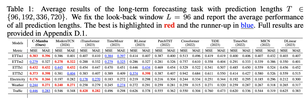
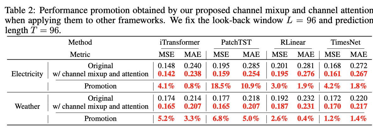
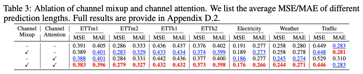
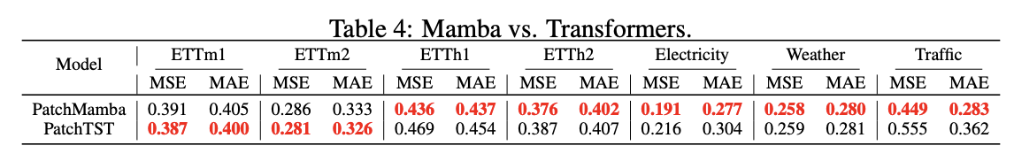
4. Experiments