AAA (All About AI)

Traffic Transformer : Capturing the continuity and periodicity of TS for traffic forecasting (2020)

Contents

1. Abstract
2. Introduction
3. Preliminaries
4. Proposed Architecture
   1. Transformer for capturing temporal dependencies
      1. Continuity of TS
      2. Periodicity of TS
      3. Summary of encoding
   2. GCN for capturing spatial dependency
   3. Traffic Transformer architecture

0. Abstract

Traffic Forecasting

• jointly model spatio-temporal dependencies

• (common) use GNN

Traffic Transformer

• (a) capture the (1) continuity & (2) periodicity of TS
• (b) model spatial dependency

1. Introduction

Traffic Transformer

design 4 novel positional encoding

• to encode (1) continuity & (2) periodicity
• to facilitate the modeling of temporal dependencies in traffic data

propose 7 temporal encoding methods, by combining different strategies

2. Preliminaries

Network-wide Traffic Forecasting task

• input : weighted directed graph \(\mathcal{G}=(\mathcal{V}, \mathcal{E}, \mathbf{W})\) , \(X^{t}\)
  • \(\mathcal{V}\) : set of sensors with \(\mid \mathcal{V} \mid =N\)
  • \(\mathcal{E}\) : set of edges connecting sensors
  • \(\mathbf{W} \in \mathbb{R}^{N \times N}\) : adjacency matrix, storing the distance between sensors
  • \(X^{t} \in \mathbb{R}^{N \times P}\) : feature matrix of the graph that is observed at time $$
    • \(P\) : number of features
• Goal :
  • predict \(H\) future steps : \(\mathcal{X}_{t+1}^{t+H}=F\left(\mathcal{G} ; \mathcal{X}_{t-(M-1)}^{t}\right)\)

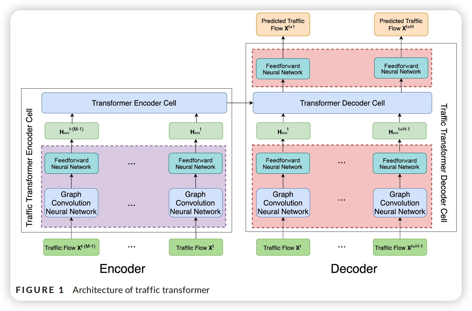
3. Proposed Architecture

• input step : [t - (M-1), \(t\) \(-(M-2), \ldots, t]\)
• output step : \([t+1, t+2, \ldots, t+H]\)

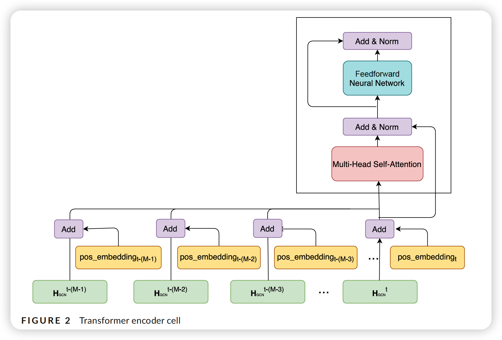
3-1. Transformer for capturing temporal dependencies

a) Continuity of TS

1. Relative Position encoding

   • continuity of time in the window ( not whole series )
   • time step \((t-(M-1))\) = starting position ( position 0 )

2. Global Position encoding

   • problem of “Relative Position encoding” : ignores the fact that most time-steps in 2 consecutive source-target sequence pairs are common

   • thus, additionally propose a global psotion

     ( has only 1 position embedding, even if it appears in different sequences )

b) Periodicity of TS

• time seires also conveys periodicity ( weekly / daily )
• 2 ways to go about this
  • (1) position encoding
  • (2) using different TS segments ( correspoing to different temporal features )

1. Periodic Position encoding
   • ex) daily-periodic embedding
   • ex) weekly-periodic position embedding

2. Time Series segment

   • ex) daily-periodic segment

     • \(\mathcal{X}_{t+1}^{t+H}(D=d)=\left[\mathcal{X}_{t+1-s d}^{t+H-s d}, \mathcal{X}_{t+1-s(d-1)}^{t+H-s(d-1)}, \ldots, \mathcal{X}_{t+1-s}^{t+H-s}\right]\).

   • ex) weekly-periodic segment

     • \(\mathcal{X}_{t+1}^{t+H}(W=w)=\left[\mathcal{X}_{t+1-s 7 w}^{t+H-s 7 w}, \mathcal{X}_{t+1-s 7(w-1)}^{t+H-s 7(w-1)}, \ldots, \mathcal{X}_{t+1-s 7}^{t+H-s 7}\right]\).

   • ex) hybrid segment

     • \(\left[\mathcal{X}_{t+1}^{t+H}(W), \mathcal{X}_{t+1}^{t+H}(D), \mathcal{X}_{t-(M-1)}^{t}\right]\).

     • Transformer can not determine the order information( \(\because\) attention based )

       \(\rightarrow\) position encoding strategy is required!

c) Summary of encoding

• 7 different encoding methods

• after obtaining position idexes…

  • method 1) addition-based combination

    • but they have different vector space!

  • method 2) similarity-based combination

    • adjust the attention score \(a_{ij}\),

      by using the similarity between 2 time steps in terms of PE

    • \(\mathbf{Y}^{i}=\sum_{j=1}^{L} a_{i j}^{\prime}\left(\mathbf{X}^{j} W_{V}\right)\).

      • \(a_{i j}^{\prime}=\frac{\exp \left(e_{i j}^{\prime}\right)}{\sum_{k=1}^{L} \exp \left(e_{i k}^{\prime}\right)}\).
        • \(e_{i j}^{\prime}=b_{i j} e_{i j}\).
          • \(d_{i j}=\text{pos embedding}_{i} \times\left(\text{pos embedding }_{j}\right)^{T}\).

3-2. GCN for capturing spatial dependency

in spectral graph theory…

• graph is represented by its Laplacian matrix
• \(g_{\theta \mathcal{G}} \mathbf{X}=\mathbf{U}_{\theta}(\boldsymbol{\Lambda}) \mathbf{U}^{T} \mathbf{X}\).
  • \(\mathbf{U} \in \mathbb{R}^{N \times N}\) : matrix of eigenvectors, decomposed from \(L\)
    • \(L=I_{N}-D^{-\frac{1}{2}} A D^{-\frac{1}{2}}=U \Lambda U^{T} \in \mathbb{R}^{N \times N}\) : normalized graph Laplacian
    • \(\mathbf{D} \in \mathbb{R}^{N \times N}\) : diagonal degree matrix
    • \(\Lambda\) : diagonal matrix of its eigen values

computationally expensive to directly decompose Laplacian matrix

use several approximations

• ex) approximate \(g_{\theta}\) with truncated expansion of Chebyshev polynomials

  • adopt first-order polynomials as the GC filter

  • stack multiple NN

  • structural neighborhood information on graphs can be incorporated by DNN,

    wihtout explicitly parameterizing polynomials

  • (before) \(g_{\theta \mathcal{G}} \mathbf{X}=\mathbf{U}_{\theta}(\boldsymbol{\Lambda}) \mathbf{U}^{T} \mathbf{X}\)

  • (after) \(g_{\theta}{ }_{G} \mathbf{X}=\theta_{0} \mathbf{X}-\theta_{1} \mathbf{D}^{-\frac{1}{2}} \mathbf{A} \mathbf{D}^{-\frac{1}{2}} \mathbf{X}\)

  • (after2) \(g_{\theta G} \mathbf{X}=\theta\left(\mathbf{I}_{N}+\mathbf{D}^{-\frac{1}{2}} \mathbf{A} D^{-\frac{1}{2}}\right) \mathbf{X}=\theta\left(\widehat{D}^{-\frac{1}{2}} \widehat{A} \widehat{D}^{-\frac{1}{2}}\right) \mathbf{X}\)

    • to reduce the number of params,
    • \(\theta\) is used to replace \(\theta_0\)
    • \(\theta=\theta_{0}=-\theta_{1}\).

\(k\)-step truncated stationary distn \(\mathcal{P}\)

\(g_{\theta}{ }_{G} \mathbf{X}=\sum_{k=0}^{K-1}\left(\theta_{k, 1}\left(\mathbf{D}_{\text {out }}^{-1} \mathbf{W}\right)^{k}+\theta_{k, 2}\left(\mathbf{D}_{\text {in }}^{-1} \mathbf{W}^{T}\right)^{k}\right) \mathbf{X}\).

• \(\theta \in \mathbb{R}^{K \times 2}\) : parameters of bidirectional filter \(g_{\theta}\)
• \(\mathbf{D}_{\text {out }}^{-1} \mathbf{W}\) and \(\mathbf{D}_{\text {in }}^{-1} \mathbf{W}^{\top}\) are the state transition matrices of the diffusion process.

3-3. Traffic Transformer architecture

Loss Function :

\(\text { Loss }=\frac{1}{H} \sum_{t=1}^{H} \frac{1}{N} \sum_{j=1}^{N} \mid X_{j}^{t}-\hat{X}_{j}^{t} \mid\).