AAA (All About AI)

Enhancing Represnetation Leanring for Periodic TS with Floss: A Frequency Domain Regularization Approach

Contents

1. Abstract
2. Introduction
3. Preliminaries
4. Method
   1. Periodic Detection & Augmentation
   2. Hierarchical Frequency-domain Loss

Abstract

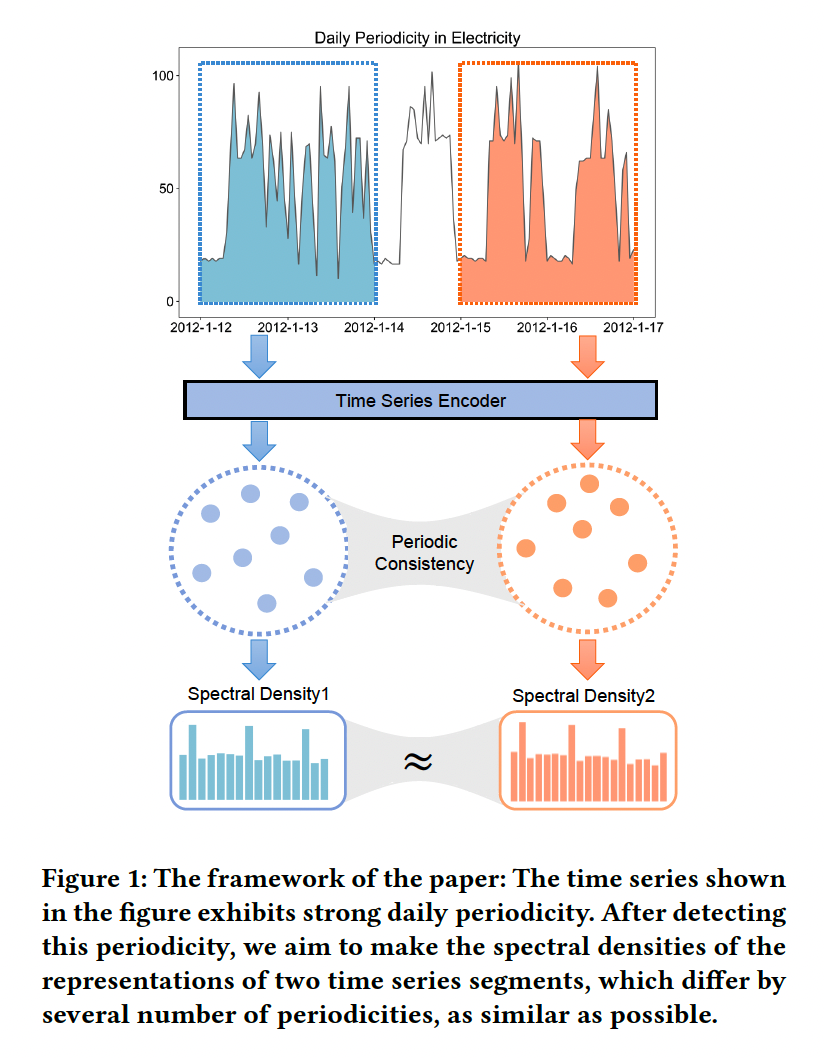
TS data exhibit periodicity

Propose an unsupervised method, “Floss”

• Automatically regularizes representations in the frequency domain

• Step 1) Automatically detect major periodicity

• Step 2) Employs periodic shift & spectral densitiy similarity measures

  \(\rightarrow\) learn representations with periodic consistency

• Easily incorporated in to both supervised / semi-supervised / unsupervised learning

1. Introduction

Temporal dynamics of real-world process: have periodicity

Classical approach to detect periodicity

• Employment of frequency domain methods
  • ex) discrete Fourier fransform (DFT)

Frequency domain information has been widely leveraged in DL arrchitectures

\(\rightarrow\) Still, none of them are specifically designed to capture periodic cynamics

Floss

• Novel approach that leverages the principles of contrastive learning (CL)
• Floss = simple yet effective combination of loss function & transformation
• (Hypothesis) Spectral density of learned representation remains invariant under periodic transformations

Details

• (1) Frequency domain transformation
  • To automatically detect dominant periodicity
• (2) Random periodic shifts
  • To create a periodic view of thee target TS in temporal dimension
• (3) Novel task
  • Enforces the similarity of spectral densities btw the target TS and its periodicc views
• (4) Hierarchical loss

2. Preliminaries

Notation

• TS: \(\mathcal{X} \in \mathbb{R}^{N \times T \times F}\), \(\mathcal{X}_{\left[t_1, t_2\right]} \in \mathbb{R}^{N \times\left(t_2-t_1+1\right) \times F}\)
• Representation model: \(\mathcal{G}(\cdot ; \theta)\)
• Representation tensor: \(\mathcal{Y}_{\left[t_1, t_2\right]}=\mathcal{G}\left(\chi_{\left[t_1, t_2\right]} ; \theta\right)\).
  • \(\mathcal{Y}_{\left[t_1, t_2\right]} \in \mathbb{R}^{N^{\prime} \times\left(t_2-t_1+1\right) \times F^{\prime}}\),

Power Spectral Density

• Provides information about the expected signal power at different frequencies of the signal
• ex) Periodogram
  • Measure of spectral density in the Fourier domain
  • discrete Fourier transform as \(\mathcal{D} \mathcal{F T}(\cdot)\),
  • Periodogram \(\Phi(\cdot)\) :
    • \(\begin{gathered} \mathcal{D} \mathcal{F} \mathcal{T}\left(w_j\right)=\frac{1}{\sqrt{n}} \sum_{t=1}^n x_t e^{-2 \pi i w_j t} \\ \Phi\left(w_j\right)=\operatorname{Re}\left(\mathcal{D} \mathcal{F T}\left(w_j\right)\right)^2+\operatorname{Im}\left(\mathcal{D} \mathcal{F} \mathcal{T}\left(w_j\right)\right)^2 \end{gathered}\).
• Other transformations are also OK
  • ex) discrete cosine transform (DCT), wavelet transform (DWT)

3. Method

Two key steps

• (1) Periodicity detenction module
• (2) Novel objective

(1) Periodic Detection & Augmentation

Identify underlying periods!

• by calculating the average spectral density

Average spectral density

\(\begin{array}{r} \hat{\Phi}=\frac{1}{N F} \sum_{n=1}^N \sum_{f=1}^F \Phi_{\mathrm{n}, \mathbf{f}}, \\ \hat{w}=\arg \max (\hat{\Phi}), \\ \hat{p}_{\left[t_1, t_2\right]}=\frac{\left(t_2-t_1+1\right)}{\hat{w}} . \end{array}\).

• \(\Phi_{\mathrm{n}, \mathrm{f}}\): Estimated periodogram of the \(f\)-th feature of the \(n\)-th TS
• \(\hat{\Phi} \in \mathbb{R}^{t_2-t_1+1}\) : Average periodogram across features.
  • \(j\)-th value \(\Phi\left(w_j\right)\) = Intensity of the frequency- \(j\) periodic basis function
    • with the period length \(\frac{\left(t_2-t_1+1\right)}{w_j}\).
• \(\hat{p}_{\left[t_1, t_2\right]}\) : Maximum periodicity = highest value observed in \(\hat{\Phi}\).

Compute periodogram for each sampled batch

• involves random sampling over time domain during the training period

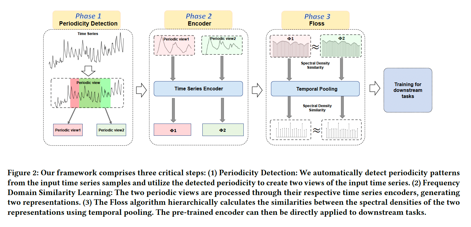
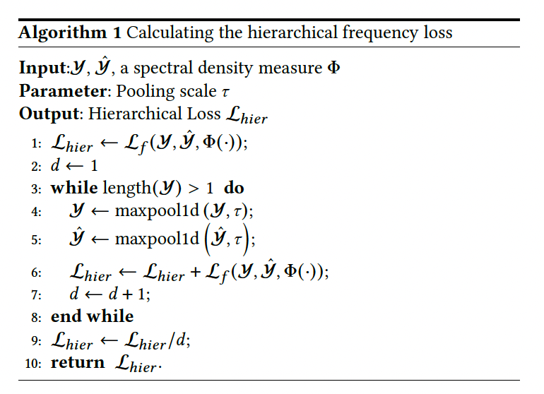
(2) Hierarchical Frequency-domain Loss

Notation

• \(\boldsymbol{y}=\mathcal{G}\left(x_{\left[t_1, t_2\right]} ; \theta\right)\) and \(\hat{\boldsymbol{y}}=\mathcal{G}\left(x_{\left[\hat{t}_1, \hat{t}_2\right]} ; \theta\right)\).
• Let \(\Phi_y\) and \(\Phi_{\hat{y}}\) : Estimated periodograms of \(\boldsymbol{y}\) and \(\hat{y}\) respectively

Loss function

• \(\mathcal{L}_f=\frac{1}{N^{\prime} F^{\prime}}\mid \mid \Phi y-\Phi_{\hat{y}}\mid \mid _{l 1}\).