AAA (All About AI)

TwinS: Revisiting Non-Stationarity in MTS Forecasting

Contents

1. Abstract
2. Introduction
3. Related Works
4. TwinS

0. Abstract

TS: Non-stationary distribution

• Time-varying statistical properties
• 3 key aspects:
  • (1) Mested periodicity
  • (2) Absence of periodic distributions
  • (3) Hysteresis among time variables

(Transformer-based) TwinS

Wavelet analysis

Address the non-stationary periodic distributions

• (1) Wavelet Convolution
  • Goal: models nested periods
  • How: by scaling the convolution kernel size like wavelet transform.
• (2) Period-Aware Attention
  • Goal: guides attention computation
  • How: generating period relevance scores through a convolutional sub-network
• (3) Channel-Temporal Mixed MLP
  • Goal: captures the overall relationships between TS
  • How: through channel-time mixing learning.

1. Introduction

Non-stationary TS

• Persistent alteration in its statistical attributes (e.g., mean and variance)

• Joint distribution across time

\(\rightarrow\) Diminishing its predictability

RevIN: TS pre-processing techniques

How about modeling the non-stationary period distribution?

• leverage the Morlet wavelet transform on the Weather dataset

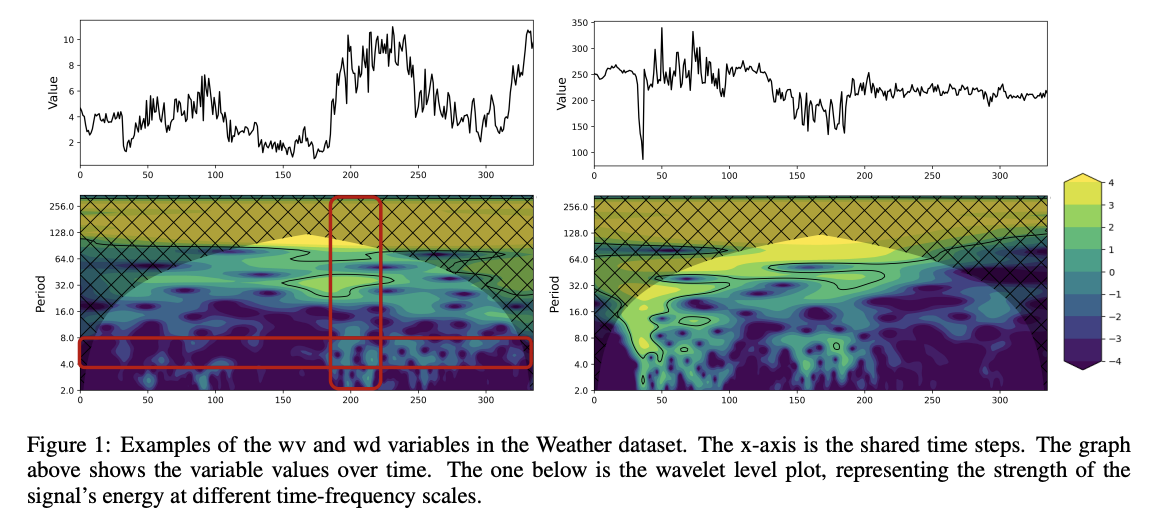
Observation (Challenges)

1. Non-stationary TS comprises “multiple nested and overlapping” periods
2. Non-stationary TS exhibit “distinct periodic patterns” segmented
   • indicating that a particular occurrence may only happen during specific stages or time intervals.
   • ex) periodicity (4~8) & time(180~330)
3. Within TS, there are similarities in the period components but significant hysteresis in periodic distribution.

Existing methods…

Challenges 1

• How: Model TS from multiple scales using various techniques

• Limitation: Only decouple the TS information in the temporal domain ( not in the frequency domain )

Challenges 2

• How: explicitly model period information through the values of each time step
• Limitation: Incorrectly aggregate noise data

Challenges 3

• Both CI & CD models neglect the hysteresis among different TS

Therefore, designing a model that can …

• (1) Decouple nested periods
• (2) Model missing states of periodicity
• (3) Capture interconnections with hysteresis among TS

are the keys factors!!

TwinS

• (1) Wavelet Convolution Module
  • Extract information from multiple nested periods
• (2) Periodic Aware (PA) Attention Module
  • Convolution-based scoring sub-network
  • Effectively models non-stationary periodic distributions at various window scales
• (3) Channel-Temporal Mixer Module
  • Treats the TS as a holistic entity
  • Employs a MLP to capture overall correlations among time variables

Contributions

1. Recognized that the critical factor for improving the performance of transformer models lies in …

   • (1) addressing nested periodicity
   • (2) modeling missing states in non-stationary periodic distribution
   • (3) capturing inter-relationships with hysteresis among MTS

2. TwinS = a novel approach that incorporates ..

   • (1) Wavelet Convolution
   • (2) Periodic Aware Attention
   • (3) Temporal-Channel Mixer MLP

   to model nonstationary period distribution;

3. Experiments

2. Related Works

CD vs. CI

CD strategy: often faces challenges such as …

• (1) prediction distribution bias (Han et al., 2023)

• (2) variations in the distributions of variables.

\(\rightarrow\) CI = generally more robust

TwinS = CI strategy category

( + possesses the capability to learn the relationships between TS )

3. TwinS

Notation

• \(\mathbf{x}_t \in \mathbb{R}^C\) .
• Input : \(\mathbf{X}_t=\left[\mathbf{x}_t, \mathbf{x}_{t+1}, \cdots, \mathbf{x}_{t+L-1}\right] \in \mathbb{R}^{C \times L}\)
• Output : \(\mathbf{Y}_t=\left[\mathbf{x}_{t+L}, \cdots, \mathbf{x}_{t+L+T-1}\right] \in \mathbb{R}^{C \times T}\)

Goal:

• Learn a mapping \(f(\cdot): X_t \rightarrow Y_t\)

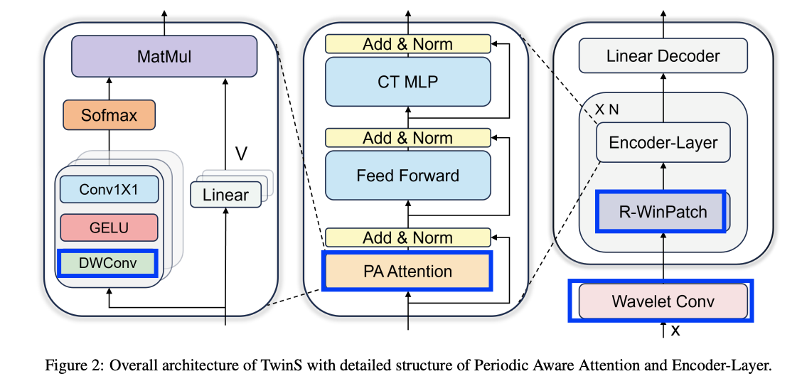
• Step 1) Wavelet convolution
  • For multi-period embedding.
• Step 2) R-WinPatch ( = Reversible window patching )
  • Capture periodicity gaps across different window scales.
• Step 3) Encoder
  • 3-1) Periodic Aware (PA) Attention
  • 3-2) Feed-forward network
  • 3-3) Channel-Temporal Mixer MLP

(1) Wavelet Convolution Embedding

Pros of “Patching”

• (1) Addresses the lack of semantic significance in individual time points
• (2) Reduces time complexity

Three concerns of patching

• (1) Does not effectively address the issue of nested periods in the TS
• (2) Important semantic information may become fragmented across different patches
  • (3) Predetermined patch length are irreversible in subsequent modeling.

Wavelet transform (WT)

Embed the TS at distinct frequency and time scales

\(W T(a, \tau, t)=\frac{1}{\sqrt{a}} \int_{-\infty}^{\infty} f(t) \cdot \psi\left(\frac{t-\tau}{a}\right) d t\).

• \(\psi\) : wavelet basis function
• \(a\) : scale parameter
  • scale of the wavelet basis functions
  • capture different frequency-domain information
• \(\tau\) : translation parameter
  • movement of the wavelet basis functions
  • capture variations in the time domain

Gabor transforms (GT) vs. Standard CNN

CNN

• = Discrete Gabor transforms (GT)
• = perform windowed Fourier transforms in the time domain on input features

\(\begin{gathered} G T(n, \tau, t)=\int_{-\infty}^{+\infty} f(t) \cdot g(t-\tau) \cdot e^{i n t} d t, \\ \operatorname{Conv}(c, k, x)=\sum_{j=1}^c \sum_{p_k \in \mathcal{R}} x\left(p_k\right) \cdot \mathbf{W}_j\left(p_k\right), \end{gathered}\).

• \(n\) : number of frequency coefficients

• \(\tau\) : translation parameter
• \(c\) : number of CNN channels
• \(k\): kerneel sizee
• \(p_k \in \mathcal{R}\) : all the sampled points in windowed kernel size
• \(g(\cdot)\): Gabor function to scale the basis function in window size
• \(\mathbf{W}_j\) : kernel weight of channel \(j\).

Difference

• GT) \(g\): typically a Gaussian function
• CNN) \(\mathbf{W}_j\) : represents trainable weights
  • automatically updated through backpropagation.

Wavelet vs. Gabor transform

• Wavelet: \(W T(a, \tau, t)=\frac{1}{\sqrt{a}} \int_{-\infty}^{\infty} f(t) \cdot \psi\left(\frac{t-\tau}{a}\right) d t\).

• Gabor: \(G T(n, \tau, t)=\int_{-\infty}^{+\infty} f(t) \cdot g(t-\tau) \cdot e^{i n t} d t\).

Key difference: “scaling factor” \(a\)

• Allows for a variable window in the Gabor transform

\(\rightarrow\) Propose Wavelet Convolution

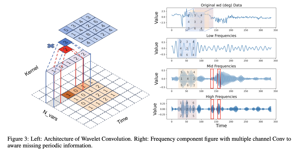
• Scaling transformations to the kernel size

  = Scaling transformations of wavelet basis functions.

• Exponentially modify the size of the convolutional kernel by power of 2 and subtract 1

  • to ensure it remains an odd number

  • Different scales ( of kernel ): share the same set of parameters \(\mathbf{W}\)

    ( = resembling the concept that wavelet functions in the wavelet transform are derived from the same base function )

\(W \operatorname{Conv}(c, k, x)=\sum_{j=1}^c \sum_{\mathbf{W}_{i j} \in \mathbf{W}} \sum_{p_k \in \mathcal{R}_i} x\left(p_k\right) \cdot \mathbf{W}_{i j}\left(p_k\right)\).

• \(p_k \in \mathcal{R}_i\) : sampled points for the kernel
  • in \(i\) th frequency scale and \(j\) th channel
• Effectively captures small-scale periodic information nested within larger periods in a TS & utilizes additive concatenation to store them

DLinear vs. Wavelet Convolution

• Recent models (DLinear) : Trend decomposition methods
  • Trend component of a time series is separately modeled using linear layers
• Wavelet convolution
  • Incorporates both information across different frequency scales and the overall trend information.

\(\mathbf{X}_{\text {point }}=W \operatorname{Conv}(\mathbf{X})+\mathbf{E}_{\text {pos }}\).

• Input: MTS data \(\mathbf{X} \in \mathbb{R}^{1 \times C \times L}\)
• Output: (1) + (2)
  • (1) Feature map of point embedding \(\mathbf{X}_{\text {point }} \in \mathbf{R}^{d \times C \times L}\)
  • (2) 1D trainable position embedding \(\mathbf{E}_{\text {pos }} \in \mathbf{R}^{d \times C \times L}\)

(2) Periodic Modeling

a) Reversible Window Patching

Inspired by the window attention mechanism in Swinformer

This paper

= combine (1) Window attention + (2) PatchTST

Details

• a) Point embedding by Wavelet Convolution
• b) Patching operations using a specific window scale
  • Merge time steps within each window for subsequent attention calculations.

Effectively handle non-stationary periodic distributions across various scales

\(\begin{gathered} \left.\mathbf{X}_{\text {patch }}^l=\text { Transpose (Unfold }\left(\mathbf{X}_{\text {point }}, \text { scale }^l, \text { stride }^l\right)\right) \\ \left.\mathbf{X}_{\text {point }}^l=\text { Transpose (Fold }\left(\mathbf{X}_{\text {patch }}, \text { scale }^l, \text { stride }^l\right)\right) \end{gathered}\).

• \(\mathbf{X}_{\text {patch }}^l \in \mathbf{R}^{C \times P^l \times D^l}\) : the patched feature map

Intra-layer window rotation operations

• on \(P\) dimension with size \(r\)
• preserve overall periodicity while improving the model’s ability to resist outliers:

\[\mathbf{X}_{\text {patch }}^l=\operatorname{Roll}\left(\mathbf{X}_{\text {patch }}, \text { shift }=r, \operatorname{dim}=P\right) .\]

b) Periods Detection Attention

MHSA block (with \(M\) heads)

• \(q=x \mathbf{W}_q, k=x \mathbf{W}_k, v=x \mathbf{W}_v\).
• \(\hat{x}=\mathbf{W}_o \cdot \operatorname{Concat}\left[\sum_{m=1}^M \sigma\left(\frac{q^{(m)} \cdot k^{(m) T}}{\sqrt{D / M}}\right) \cdot v^{(m)}\right]\).

Limitataion of MHSA:

• TS exist multiple non-stationary periods

( Refer to Figure 3-right )

• Ideal) Attention score
  • (High frequency) T=160 > T=140
  • (Midd frequency) T=140: may exhibit a period of absence

[ Deformable methods ]

• Deformable convolution (Dai et al., 2017)

• Deformable attention (Zhu et al., 2020; Xia et al., 2022)

\(\rightarrow\) Utilizes a sub-network to adaptively adjust the receptive field shape by fine-grained feature mapping,

Proposal: Convolution sub-network to aware “periodicity absence” with their translation invariance

\(\rightarrow\) Guide the information allocation in attention computation.

Details

• Follow the principle of “multi-head”

• Employ multi-head Periodic Aware sub-network

  • To generate multiple periodic score matrices
  • Enable each channel of the Conv to independently focus on a specific periodic pattern based on multiple periodic feature map embedded

• Employ MLP to aggregate the information from multiple channels within an aware head

  \(\rightarrow\) Obtain the periodic relevance scores

Periodic relevance scores

\(\mathbf{W}_{\text {score }}^{(l s)}=\operatorname{sigmoid}(\mathbf{W}_p \cdot \sigma(D W \operatorname{Conv}(\mathbf{X}_{\text {patch }}^{(l)})^{(s)})\).

• DWConv: Depthwise Separable Convolution (Chollet, 2017)
  • utilized to detect periodic missing states

\(\hat{\mathbf{X}}_{\text {patch }}^l=\mathbf{W}_o \cdot \operatorname{Concat}\left[\sum_{m=1}^M \sigma\left(\frac{\mathbf{W}_{\text {score }}^{(l m)} \cdot q^{(l m)} \cdot k^{(l m) T}}{\sqrt{D_l / M}}\right) \cdot v^{(l m)}\right]\).

Simpler!! Discard the keys

( = Directly use the lightweight sub-network to generate the attention matrix based on the query )

\(\hat{\mathbf{X}}_{\text {patch }}^l=\mathbf{W}_o \cdot \text { Concat }\left[\sum_{m=1}^M \sigma\left(\mathbf{W}_{\text {score }}^{(l m)}\right) \cdot v^{(l m)}\right]\).

(3) Channel-Tepomral Mixer MLP

Capturing relationships between channels (variables)

• Enhance model performance (Zhang \& Yan, 2022)

Several models (Yu et al., 2023; Chen et al., 2023)

• separate modeling of dependencies in channel and time dimensions

Channel attention

• Model the variable relationships at each time step

\(\rightarrow\) Distribution hysteresis can incorrectly model the relationship information!

Solution: Adopt a joint learning approach

( instead of isolated modeling channels and time dependencies )

\(\hat{\mathbf{H}}_{\text {patch }}^l=\mathbf{W}_2 \cdot \sigma\left(\mathbf{W}_1 \cdot \mathbf{H}_{\text {patch }}^l+b_1\right)+b_2\).

• \(\mathbf{H}_{\text {patch }}^l \in \mathbf{R}^{D^l \times\left(C P^l\right)}\) : channel-temporal mixer representation
  • via reshape with \(\mathbf{X}_{\text {patch }} \in \mathbf{R}^{C \times P^l \times D^l}\)
• \(\mathbf{W}_1 \in \mathbf{R}^{D^l \times h}\) and \(\mathbf{W}_2 \in \mathbf{R}^{h \times D^l}\)