AAA (All About AI)

Leveraging 2D Information for Long-term Time Series Forecasting with Vanilla Transformers

Contents

1. Abstract
2. Introduction
3. GridTST
   1. Problem Formulation
   2. Model Structure

0. Abstract

TS Transformer architecture:

• Approach 1) Encoding multiple variables from the same timestamp into a single temporal token to model global dependencies
• Approach 2) Embeds the time points of individual series into separate variate tokens

Limitations:

• Approach 1) Challengees in variate-centric representations

• Approach 2) Risks missing essential temporal information critical for accurate forecasting.

GridTST

• Combines the benefits of two approaches
• Multi-directional attentions
• Input TS = Grid
  • (x-axis) Time steps
  • (y-axis) Variates.
• Slicing
  • Vertical slicing: combines the variates at each time step into a time token
  • Horizontal slicing: embeds the individual series across all time steps into a variate token
• Attention
  • Horizontal attention : focuses on time tokens
    • to comprehend the correlations between data at various time steps
  • Vertical, variate-aware attention : grasp multivariate correlations

\(\rightarrow\) Enables efficient processing of information across both time and variate dimensions

1. Introduction

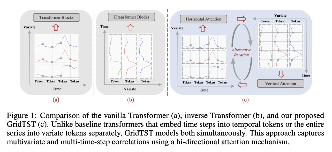
Figure 1(a): Classic transformer

• Embed multi-variate data points from the same timestamp into a single variable
• Limitation
  • Single-time-step tokens may not effectively convey information due to their limited receptive field
  • Inappropriate use of permutation-invariant attention in the temporal dimension

Figure 1(b): iTransformer

• Inverts the roles of the attention mechanism and FFN
• Representing time points as “variate tokens”
• Limitation
  • Still lacks adequate timestamp modeling

Question: Can the vanilla Transformer architecture effectively capture both temporal and covariate information?

GridTST

Captures the (1) cross-time and (2) cross-variate dependency

• By adapting the traditional attention mechanism and architecture from different views

Details: Figure 1(c)

• (1) Patching
• (2) Visualize the input TS as a grid
  • (x-axis) Time steps \(\rightarrow\) time token
  • (y-axis) Variates \(\rightarrow\) vaariate token
• (3) Attention
  • Horizontal attention:
    • on time tokens to analyze correlations between data at different time steps
  • Vertical attention:
    • to capture the multivariate correlations

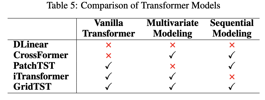
Contributions

1. Findings: Both temporal and covariate information are crucial for the task of time series prediction.
2. GridTST: Leverages the foundational Transformer architecture
   • capture both temporal dynamics and covariate info
3. SOTA on real-world forecasting benchmarks

2. GridTST

(1) Problem Formulation

Notation

• Input: \(X=\) \(\left\{x_1, \ldots, x_T\right\} \in \mathbb{R}^{T \times N}\),
• Target: \(Y=\left\{x_{T+1}, \ldots, x_{T+F}\right\} \in\) \(\mathbb{R}^{F \times N}\).
• Prediction: \(\hat{Y}=\left\{\hat{x}_{T+1}, \ldots, \hat{x}_{T+F}\right\} \in \mathbb{R}^{F \times N}\).

(2) Model Structure

GridTST

• Vanilla encoder-only architecture of Transformer
• Patched embedding, horizontal and vertical attentions

a) Patched Time Tokens

Use patching

( \(\because\) Single time step does not convey semantic value! )

[Procedure]

**(Step 1) Input UTS: \(X_{:, n} \in \mathbb{R}^{T \times 1}\) **

(Step 2) Segment into patches

• Patch size = \(P\)
• Result: \(X_{i, n}^p \in \mathbb{R}^{M \times P}\),
  • Total number of patches: \(M=\left\lceil\frac{T-P}{S}\right\rceil+2\).

• To maintain continuity at the boundary, we append \(S\) copies of the final value \(X_{T, n} \in \mathbb{R}\) to the sequence before initiating the patching process.

• Memory usage & computational complexity of the attention map are quadratically decreased by a factor of \(S\).

(Step 3) Projection

• Project to dimension \(D\) , using
  • a trainable linear projection \(W_p \in \mathbb{R}^{P \times D}\),
  • a learnable additive position encoding \(W_{\text {pos }} \in \mathbb{R}^{M \times D}\),
• \(X_{:, n}^d=X_{i, n}^p W_p+W_{\text {pos }}\),
  • where \(X_{:, n}^d \in \mathbb{R}^{M \times D}\)

(Step 4) Define the grid

• Input grid: \(X^d=\left\{X_1^d, \ldots, X_M^d\right\} \in \mathbb{R}^{M \times N \times D}\).
  • \(X_{t,:}^d \in \mathbb{R}^{N \times D}\) : MTS encapsulated within the patch at step \(t\),
  • \(X_{:, n}^d \in \mathbb{R}^{M \times D}\) : Complete patched TS corresponding to the \(n\)-th variate

b) Horizontal Attention (TIME)

Captures the sequential nature and temporal dynamics in TS

Example) \(n\)-th variate series

• Horizontal attention on the patched time tokens \(X_{:, n}^d \in \mathbb{R}^{M \times D}\)
• MHSA) Head \(h=\{1, \ldots, H\}\) transforms these inputs into…
  • (1) Query matrices \(Q_{:, n}^h=X_{:, n}^d W_h^Q\)
  • (2) Key matrices \(K_{:, n}^h=X_{:, n}^d W_h^K\)
  • (3) Value matrices \(V_{:, n}^h=X_{:, n}^d W_h^V\)
    • where \(W_h^Q, W_h^K \in \mathbb{R}^{D \times d_k}\) and \(W_h^V \in \mathbb{R}^{D \times D}\).
• Attention output \(O_{:, n}^d \in \mathbb{R}^{M \times D}\) :
  • \(O_{:, n}^d=\operatorname{Attention}\left(Q_{:, n}^h, K_{:, n}^h, V_{:, n}^h\right)=\operatorname{Softmax}\left(\frac{Q_{:, n}^h\left(K_{:, n}^h\right)^T}{\sqrt{d_k}}\right) V_{:, n}^h\).
• BN & FFN ( + Residual connection )
  • \(O_{:, n}^{d, l}=\operatorname{Attn}_{\text {horizontal }}\left(O_{:, n}^{d, l-1}\right)\).
    • \(l\): layer index

c) Vertical Attention (VARIATE)

Capture the relationships between different variates (at a given time step)

Use variate tokens \(X_{t,:}^d \in \mathbb{R}^{N \times D}\).

Example)

• MHSA) Head \(h=\{1, \ldots, H\}\) transforms these inputs into…

  • Query matrices \(\hat{Q}_{t,:}^h=X_{t,:}^d W_h^{\hat{Q}}\),

  • Key matrices \(\hat{K}_{t,:}^h=X_{t,:}^d W_h^{\hat{K}}\),

  • Value matrices \(\hat{V}_{t,:}^h=X_{t,:}^d W_h^{\hat{V}}\).

    • whereH \(W_h^{\hat{Q}}, W_h^{\hat{K}} \in \mathbb{R}^{D \times d_k}\) and \(W_h^{\hat{V}} \in \mathbb{R}^{D \times D}\).
• Attention output: \(\hat{O}_{t,:}^d \in \mathbb{R}^{N \times D}\) :
  • \(\hat{O}_{t,:}^d=\operatorname{Attention}\left(\hat{Q}_{t,:}^h, \hat{K}_{t,:}^h, \hat{V}_{t,:}^h\right)=\operatorname{Softmax}\left(\frac{\hat{Q}_{t,:}^h\left(\hat{K}_{t, i^h}^T\right.}{\sqrt{d_k}}\right) \hat{V}_{t,:}^h\).
• BN & FFN ( + Residual connection )
  • \(\hat{O}_{:, n}^{d, l}=\operatorname{Attn}_{\text {vertical }}\left(\hat{O}_{t:}^{d, l-1}\right)\).

c) Attention Sequencing

Order of applying horizontal and vertical attentions

• (1) Time-first
• (2) Channel-first
• (3) Iterative approach

\(\rightarrow\) Discovered that the sequence starting with vertical attention and then transitioning to horizontal yields the best performance.

• vertical attention first captures complex variate relationships
• laying the groundwork for horizontal attention to then effectively grasp temporal patterns,

d) Complexity

Settings

• TS with \(m\) covariates and \(n\) patches
• Transformer model with a hidden size of \(d\).

Computational complexity of the attention layer for ..

• PatchTST: \(\mathcal{O}\left(n^2 d\right)\),
• GridTST: \(\mathcal{O}\left(\frac{m^2 d}{2}+\frac{n^2 d}{2}\right)\).

\(\rightarrow\) Datasets with a relatively small number of covariates can operate more efficiently than PatchTST.

( + For dataset with large covariate number, we also design an efficient training algorithm by variate sampling )

e) Normalization

Representation after the attention sequence:

• \(Z \in \mathbb{R}^{M \times N \times D}\).

Processed through a flatten layer (with a linear head)

Normalization

• instance normalization before patching
• instance denormalization after this linear head