AAA (All About AI)

MTS-Mixers: Multivariate Time Series Forecasting via Factorized Temporal and Channel Mixing

Contents

1. Abstract
2. Introduction
3. Preliminary
4. MTS-Mixers
5. Experiments

0. Abstract

Role of attention modules is not clear!!

Findings

• (1) Attention is not necessary for capturing temporal dependencies
• (2) Entanglement and redundancy in the capture of temporal and channel interaction affect the forecasting performance
• (3) It is important to model the mapping between the input and the prediction.

Propose *MTS-Mixers

• Two factorized modules to capture temporal and channel dependencies.

1. Introduction

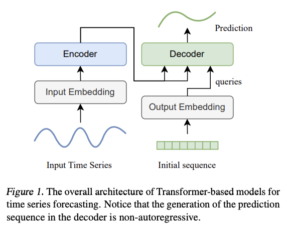
Transformer-based models

• Perform well on LTSF … Still some problems!

Limitation

• (1) Lack of explanation about the attention mechanism for capturing temporal dependency

• (2) Heavily rely on additional positional or date-specific encoding
  • May disturb the capture of temporal interaction
• (3) Bulk of additional operations beyond attention

Findings

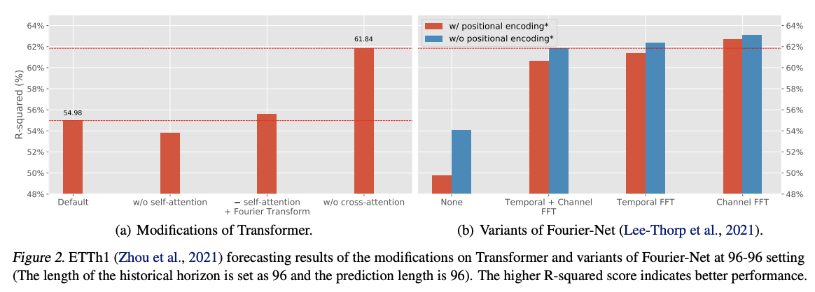
• (1) Replacing the attention layer with Fourier Transform maintains the forecasting performance
• (2) Removing the cross-attention significantly improves it.

\(\rightarrow\) Attention mechanism on TS forecasting tasks may not be that effective

Due to the difference in the sampling rate & # of sensors

\(\rightarrow\) MTS from different scenarios often vary greatly & serious redundancy

Example) \(\mathcal{X} \in \mathbb{R}^{n \times c}\)

• \(n\) : length of \(\mathcal{X}\)
• \(c\) : dimension size

\(\rightarrow\) uncertain which one (\(n,c\)) is bigger or smaller!

Generally has the low-rank property, such that \(\operatorname{rank}(\mathcal{X}) \ll \min (n, c)\).

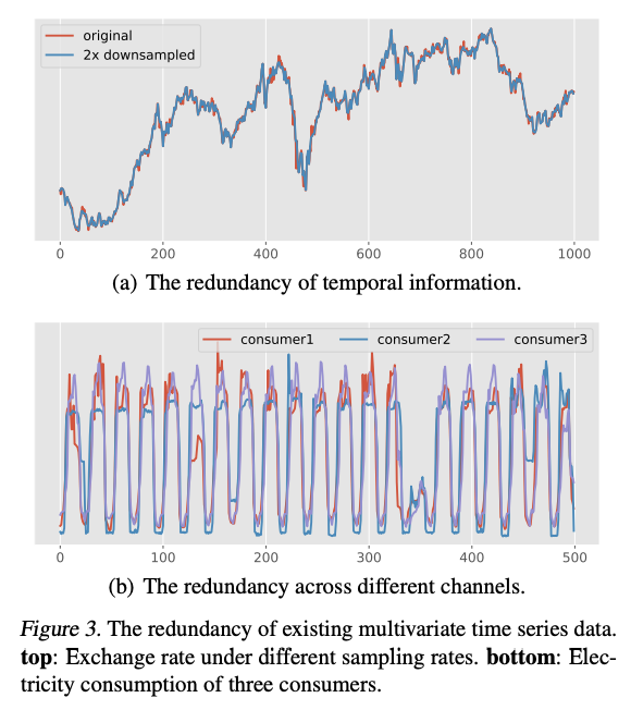
• Redundancy of temporal and channel information.

Solution: propose MTS-Mixers

Contributions

1. Investigate the attention mechanism in TS forecasting

   & Propose MTS-Mixers

   • which respectively capture temporal and channel dependencies

2. Leverage the low-rank property of existing TS via factorized temporal and channel mixing

3. Experiments

2. Preliminary

(1) Problem definition

Input TS: \(\mathcal{X}_h=\) \(\left[\boldsymbol{x}_1, \boldsymbol{x}_2, \ldots, \boldsymbol{x}_n\right] \in \mathbb{R}^{n \times c}\)

Output TS: \(\mathcal{X}_f=\left[\boldsymbol{x}_{n+1}, \boldsymbol{x}_{n+2}, \ldots, \boldsymbol{x}_{n+m}\right] \in \mathbb{R}^{m \times c}\)

• across all the \(c\) channels.

Forecasting tasks: learn a map \(\mathcal{F}: \mathcal{X}_h^{n \times c} \mapsto \mathcal{X}_f^{m \times c}\)

(2) Rethinking the mechanism of attention in Transformer-based forecasting models

Existing Transformer-based methods

• Step 1) 1D CNN for input embedding \(\mathcal{X}_{\text {in }} \in \mathbb{R}^{n \times d}\)
  • with the positional or date-specific encoding
• Step 2) Self-attention
  • Token-level temporal similarity
  • \(\tilde{\mathcal{X}}=\operatorname{softmax}\left(\frac{\mathcal{X}_{\text {in }} \cdot \mathcal{X}_{\text {in }}^{\top}}{\sqrt{d}}\right) \cdot \mathcal{X}=R_1 \cdot \mathcal{X}_{\text {in }}\).
    • where \(R_1 \in \mathbb{R}^{n \times n}\) describes token-wise temporal information.
• Step 3) FFN with two linear layers and activation function
  • to learn channel-wise features
• Step 4) Decoder
  • Initialized query \(Q \in \mathbb{R}^{m \times d}\)
  • Output: \(\tilde{\mathcal{X}}_f=\operatorname{softmax}\left(\frac{Q \cdot \tilde{\mathcal{X}}^{\top}}{\sqrt{d}}\right) \cdot \tilde{\mathcal{X}}=R_2 \cdot \tilde{\mathcal{X}},\).
    • where \(R_2 \in \mathbb{R}^{m \times n}\) describes the relationship between the input & output
• Step 5) Projection layer
  • applied on \(\tilde{\mathcal{X}}_f\) to obtain \(\mathcal{X}_f \in \mathbb{R}^{m \times c}\).

Summary

Contain two stages:

• (1) Learning token-wise temporal dependency across channels,
• (2) Learning a map between input & output

However, as shown in Figure 2 …

\(\rightarrow\) Removing self-attention or cross-attention is still OK

3. MTS-Mixers

Notation

• Input \(\mathcal{X}_h \in \mathbb{R}^{n \times c}\)
• Output \(\mathcal{X}_f \in \mathbb{R}^{m \times c}\).

( Input embedding module is optional )

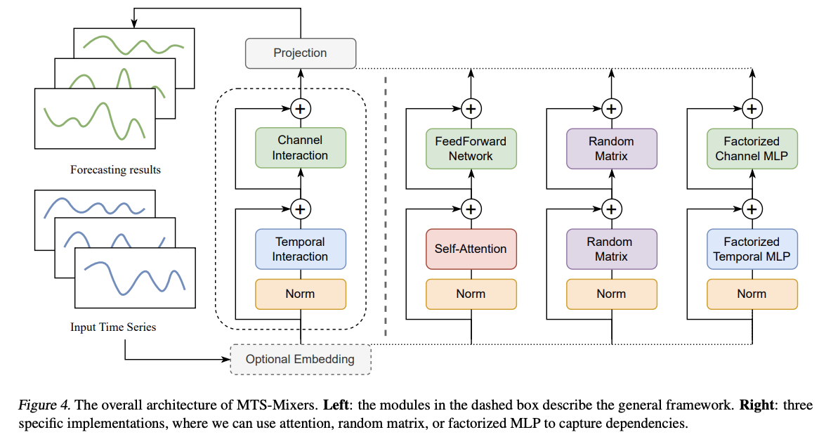
Overall Process

\(\begin{aligned} \mathcal{X}_h^{\mathcal{T}} & =\operatorname{Temporal}\left(\operatorname{norm}\left(\mathcal{X}_h\right)\right) \\ \mathcal{X}_h^{\mathcal{C}} & =\operatorname{Channel}\left(\mathcal{X}_h+\mathcal{X}_h^{\mathcal{T}}\right) \\ \mathcal{X}_f & =\operatorname{Linear}\left(\mathcal{X}_h^{\mathcal{T}}+\mathcal{X}_h^{\mathcal{C}}\right) . \end{aligned}\).

Three specific implementations

• (1) Attention-based MTS-Mixer
• (2) Random matrix MTS-Mixer
• (3) Factorized temporal and channel mixing

(1) Attention-based MTS-Mixer

\(\begin{aligned} \tilde{\mathcal{X}}_h & =\operatorname{norm}\left(\mathcal{X}_h\right)+\operatorname{PE}\left(\mathcal{X}_h\right) \\ \mathcal{X}_h^{\mathcal{T}} & =\operatorname{Attention}\left(\tilde{\mathcal{X}}_h, \tilde{\mathcal{X}}_h, \tilde{\mathcal{X}}_h\right) \\ \mathcal{X}_h^{\mathcal{C}} & =\operatorname{FFN}\left(\tilde{\mathcal{X}}_h+\mathcal{X}_h^{\mathcal{\tau}}\right) . \end{aligned}\).

Step 1) Add the sinusoidal positional encoding

\(\rightarrow\) Obtain the input embedding \(\tilde{\mathcal{X}}_h\)

Step 2) MHSA

• Capture temporal dependency \(\mathcal{X}_h^\tau\).

Step 3) FFN

• learn the channel interaction \(\mathcal{X}_h^{\mathcal{C}}\).

Step 4) Linear Layer ( NO decoder )

• directly learn the map between the input & output

(2) Random matrix MTS-Mixer

\(\mathcal{X}_f=F \cdot \sigma(T) \cdot \mathcal{X}_h \cdot \phi(C)\).

What we need to learn …

• (1) \(T \in \mathbb{R}^{n \times n}\) : the temporal dependency,
• (2) \(C \in \mathbb{R}^{c \times c}\) : the channel dependency
• (3) Projection \(F \in \mathbb{R}^{m \times n}\)

Because the initialization of the matrices \(F\), \(T\), and \(C\) are controllable

\(\rightarrow\) Call it a random matrix MTSMixer

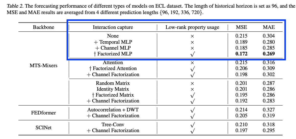
(3) Factorized temporal and channel mixing

Low rank property of TS data

\(\rightarrow\) Factorized temporal and channel mixing strategies

• to capture dependencies with less redundancy

Extract the temporal dependencies as…

\(\begin{aligned} \mathcal{X}_{h, 1}, \ldots, \mathcal{X}_{h, s} & =\operatorname{sampled}\left(\operatorname{norm}\left(\mathcal{X}_h\right)\right), \\ \mathcal{X}_{h, i}^{\mathcal{T}} & =\operatorname{Temporal}\left(\mathcal{X}_{h, i}\right) \quad i \in[1, s], \\ \mathcal{X}_h^{\mathcal{T}} & =\operatorname{merge}\left(\mathcal{X}_{h, 1}^{\mathcal{T}}, \ldots, \mathcal{X}_{h, s}^{\mathcal{T}}\right) \end{aligned}\).

• Step 1) downsample the original TS
• Step 2) Utilize one temporal feature extractor
  • (e.g., MLP or attention)
• Step 3) Merge them in the original order.

For TS with channel redundancy …

• Reduce the noise of tensors corresponding to the TSin channel dimension by “matrix decomposition”

\(\begin{aligned} \tilde{\mathcal{X}}_h^c & =\mathcal{X}_h+\mathcal{X}_h^{\mathcal{\tau}}, \\ \tilde{\mathcal{X}}_h^c & =\mathcal{X}_h^{\mathcal{C}}+N \approx U V+N, \end{aligned}\).

• \(N \in \mathbb{R}^{n \times c}\) : the noise
• \(\mathcal{X}_h^{\mathcal{c}} \in \mathbb{R}^{n \times c}\) : channel dependency after denoising
• \(U \in\) \(\mathbb{R}^{n \times m}\) and \(V \in \mathbb{R}^{m \times c}(m<c)\) : factorized channel interaction.

\(\mathcal{X}_h^{\mathcal{C}}=\sigma\left(\tilde{\mathcal{X}_h^{\mathcal{C}}} \cdot W_1^{\top}+b_1\right) \cdot W_2^{\top}+b_2,\).

• where \(W_1 \in \mathbb{R}^{m \times c}, W_2 \in \mathbb{R}^{c \times m}\)

4. Experiments