AAA (All About AI)

Revisiting Long-term Time Series Forecasting: An Investigation on Linear Mapping

Contents

1. Abstract
2. Introduction
3. Problem Definition
4. Are Temporal Feature Extractors Effective?
5. Theoretical and Empirical Study on the Linear Mapping
6. Experiments

0. Abstract

LTSF

Previous studies: single linear layer can achieve competitive forecasting performance compared to other complex architectures

3 key observations:

1. Linear mapping is critical to prior LTSF
2. RevIN (reversible normalization) and CI (Channel Independent) play a vital role in improving overall forecasting performance
3. Linear mapping can effectively capture periodic features in TS & has robustness for different periods across channels when increasing the input horizon.

\(\rightarrow\) Provide theoretical and experimental explanations!

1. Introduction

Background:

• LTSF-Linear

  • Uses only a single linear layer
  • Outperforms existing complex architectures

• Subsequent approaches [14, 18, 13, 25]

  • Discarded the encoder-decoder architecture
  • Focused on developing temporal feature extractors

  \(\rightarrow\) Still not significantly better than linear models.

  & often require a large number of adjustable hyper-parameters and specific training tricks

Raise the following questions:

• (1) Are temporal feature extractors effective for LTSF?
• (2) What are the underlying mechanisms explaining the effectiveness of linear mapping in TSF?
• (3) What are the limits of linear models & how can we improve them?

Contributions

1. We investigate the efficacy of different components in recent TSF models
   • Finding) Linear mapping is critical to their forecasting performance ( Section 3 )*
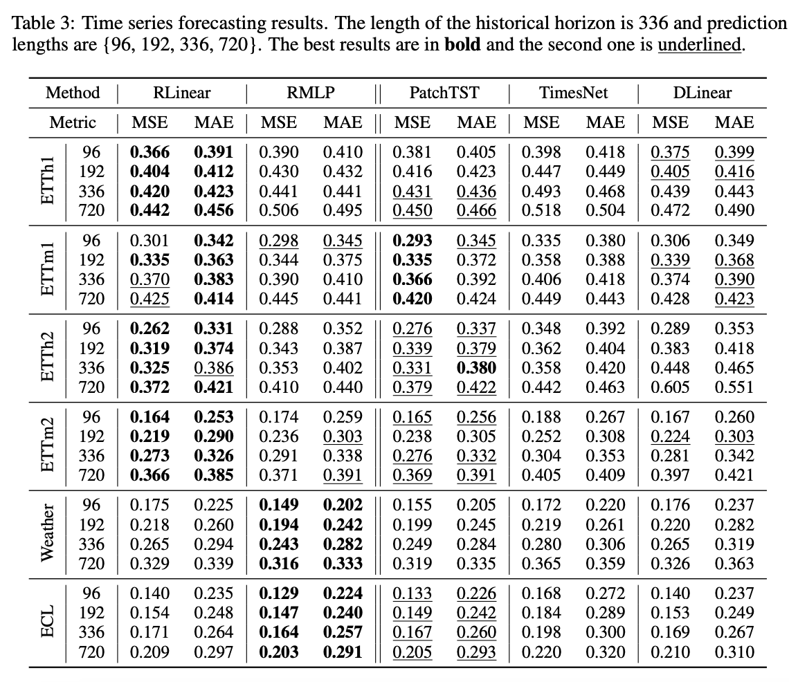
2. Demonstrate the effectiveness of linear mapping for learning periodicity in LTSF with both theoretical and experimental evidence & propose simple yet effective baselines ( Table 3 )
3. Examine the limitations of the linear mapping when dealing with MTS with different periodic channels, and analysis the impact of the input horizon and a remedial technique called Channel-Independent ( Figure 10, 11 )

2. Problem Definition

• \(\mathbf{X}=\left[\boldsymbol{x}_1, \boldsymbol{x}_2, \ldots, \boldsymbol{x}_n\right] \in \mathbb{R}^{c \times n}\) ,
• \(\mathbf{Y}=\) \(\left[\boldsymbol{x}_{n+1}, \boldsymbol{x}_{n+2}, \ldots, \boldsymbol{x}_{n+m}\right] \in \mathbb{R}^{c \times m}\) ,
• Learn a map \(\mathcal{F}: \mathbf{X}^{c \times n} \mapsto \mathbf{Y}^{c \times m}\)

3. Are Temporal Feature Extractors Effective?

General framework

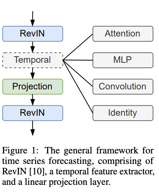
Three core components:

• (1) RevIN
• (2) Temporal feature extractor
  • such as attention, MLP, or convolutional layers
• (3) Linear projection layer
  • projects the final prediction results

(1) Temporal feature extractors

Examine the effectiveness of different temporal feature extractors

• Select four notable recent developments:
  • PatchTST [18] (attention)
  • MTS-Mixers [13] (MLP)
  • TimesNet [25] and SCINet [14] (convolution)
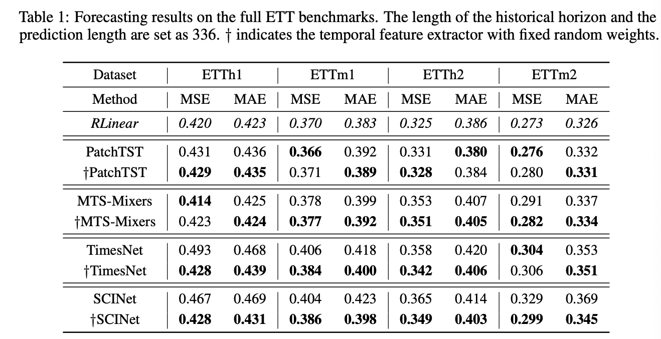
• Conduct new experiments using the ETT benchmark to check the contribution of each part

Result

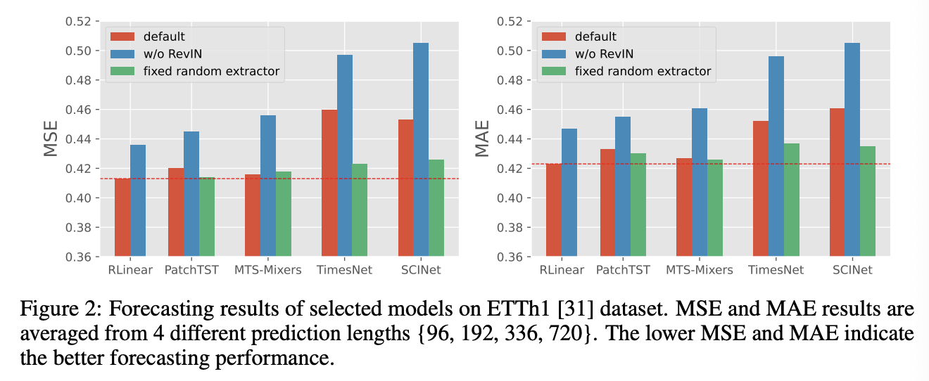
• RLinear: (baseline) refers to a linear projection layer with RevIN.
• Fixed random extractor: only initialize the temporal feature extractor randomly and do not update its parameters

Summary

• (1) RevIN significantly improves the performance
• (2) With the aid of RevIN, even a simple linear layer can outperform current SOTA baseline PatchTST.

(2) Weight Visualization

Even using a randomly initialized temporal feature extractor can induce competitive results!!!

Q) What have these feature extractorslearned from TS data??

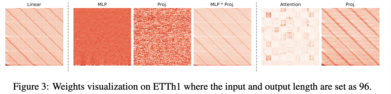
• Weights of the final linear projection layer

  with different temporal feature extractors

Summary: When the temporal feature extractor is …

• (1) MLP…

  • a) Both MLP and projection layer learn chaotic weights,
  • b) Product of the two remains consistent with the weights learned from a single linear layer

• (2) Attention…

  • a) Also learns about messy weights
  • b) But the weight learned by the projection layer is similar to that of a single linear layer

  \(\rightarrow\) Implying the importance of linear projection in TSF

4. Theoretical and Empirical Study on the Linear Mapping

(1) Roles of Linear Mapping in Forecasting

Linear mapping learns periodicity

Single linear layer: \(\mathbf{Y}=\mathbf{X} \mathbf{W}+\mathbf{b}\)

• where \(\mathbf{W} \in \mathbb{R}^{n \times m}\) & \(\mathbf{b} \in \mathbb{R}^{1 \times m}\)

Assumption 1) General TS \(x(t)\) can be disentangled into …

• seasonality part \(s(t)\) and trend part \(f(t)\)
• \(x(t)=s(t)+f(t)+\epsilon\).

It’s worth noting that a single linear layer can also effectively learn periodic patterns.

Theorem 1) Given a seasonal TS satisfying \(x(t)=s(t)=s(t-p)\) where \(p \leq n\) is the period,

there always exists an analytical solution for the linear model as

\(\left[\boldsymbol{x}_1, \boldsymbol{x}_2, \ldots, \boldsymbol{x}_n\right] \cdot \mathbf{W}+\mathbf{b}=\left[\boldsymbol{x}_{n+1}, \boldsymbol{x}_{n+2}, \ldots, \boldsymbol{x}_{n+m}\right]\).

\(\mathbf{W}_{i j}^{(k)}=\left\{\begin{array}{ll} 1, & \text { if } i=n-k p+(j \bmod p) \\ 0, & \text { otherwise } \end{array}, 1 \leq k \in \mathbb{Z} \leq\lfloor n / p\rfloor, b_i=0\right.\).

Summary

• Indicates that linear mapping can predict periodic signals when \(n \geq m\) … but not a unique solution.

• Since the values corresponding to each timestamp in \(s(t)\) are almost impossible to be linearly independent, the solution space for the parameters of \(W\) is extensive.

• Possible to obtain a closed-form solution for more potential values of \(\mathbf{W}^{(k)}\) with different factor \(k\) when \(n \gg p\).

  • ex) The linear combination of \(\left[\mathbf{W}^{(1)}, \ldots, \mathbf{W}^{(k)}\right]\) with proper scaling factor

  • Corollary 1.1. When the given TS satisfies \(x(t)=a x(t-p)+c\) where \(a, c\) are scaling and translation factors, the linear model still has a closed-form solution as

    \(\mathbf{W}_{i j}^{(k)}=\left\{\begin{array}{ll} a^k, & \text { if } i=n-k p+(j \bmod p) \\ 0, & \text { otherwise } \end{array}, 1 \leq k \in \mathbb{Z} \leq\lfloor n / p\rfloor, b_i=\sum_{l=0}^{k-1} a^l \cdot c\right.\).

(2) Disentanglement and Normalization

a) Problems in Disentanglement

If the trend term can be separated from the seasonal term, forecasting performance can be improved!

Previous works [8, 28, 26, 23, 24, 33, 29, 27]

• Focused on disentangling TS & predict them individaully

  • ex) moving average

• However, these disentanglement methods have problems [12]:

  • (1) Sliding window size should be larger than the maximum period of seasonality parts

  • (2) Usage of the average pooling layer, alignment requires padding on both ends of the input TS

    \(\rightarrow\) Distorts the sequence at the head and tail

  • (3) Even if the signals are completely disentangled …

    \(\rightarrow\) Issue of under-fitting trend terms persists.

Therefore, while disentanglement may improve forecasting performance, it still has a gap with some recent advanced models.

b) Turning trend into seasonality.

Key to disentanglement

• Subtracting the MA from original TS ( = normalization )

RevIN: Statistics of TS continuously change over time

( due to the distribution shift problem )

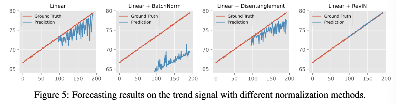
However, the range and size of values in TS are also meaningful!!

\(\rightarrow\) Directly applying normalization to input TS may erase this statistical information ( Figure 5 )

\(\rightarrow\) That’s why RevIN is good ( lies in “reversibility” )

RevIN

• Eliminates trend changes caused by moment statistics
• Preserves statistical information that can be used to restore final forecasting results.

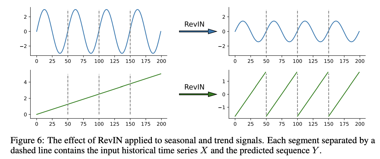
• Example) Figure 6: How RevIN affects seasonal and trend terms
  • Seasonal signal:
    • Scales the range but does not change the periodicity
  • Trend signal:
    • Scales each segment into the same range and exhibits periodic patterns.
  • RevIN is capable of turning some trends into seasonality

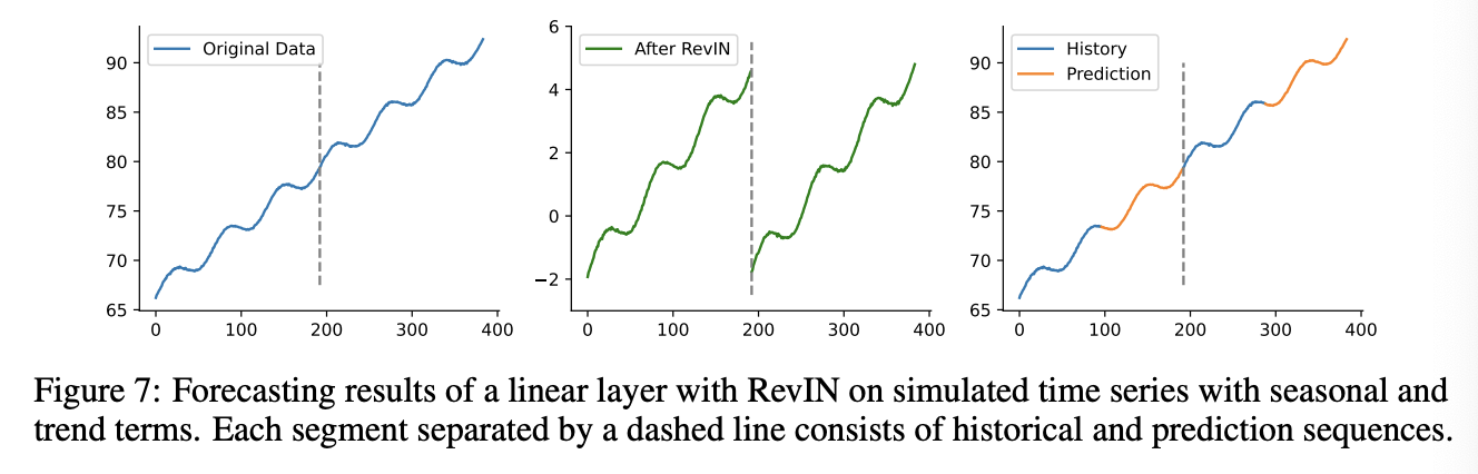
• Example) Figure 7: RevIN converts continuously changing trends into multiple segments with a fixed and similar trend, demonstrating periodic characteristics.

5. Experiments

When Linear Meets Multiple Periods among Channels??

Linear mapping

• Pros) Capable of learning periodicity in TS

• Cons) Faces challenges when dealing with multi-channel datasets.

  \(\rightarrow\) Possible solution: CI modeling

  • Treats each channel in the TS independently
    • (1) Improve performance
    • (2) Increases computational overhead
  • Result (Figure 8):
    • RLinear-CI and RMLP are able to fit curves
    • RLinear fails.

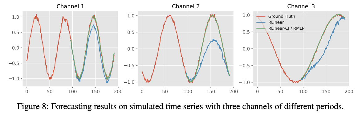
Summary

• Single linear layer may struggle to learn different periods within channels.
• Nonlinear units or CI modeling may be useful in enhancing the robustness of the model for MTS with different periodic channels.