AAA (All About AI)

CycleNet: Enhancing Time Series Forecasting through Modeling Periodic Patterns

Contents

1. Abstract
2. Introduction
3. Related Works
4. CycleNet
   1. Residual Cycle Foreacsting
   2. Backbone
5. Experiments
6. Discussion

0. Abstract

Stable periodic patterns

\(\rightarrow\) Foundation for conducting long-horizon forecasts

Residual Cycle Forecasting (RCF)

• Learnable recurrent cycles
  • To model the inherent periodic patterns
• Predictions on the residual components of the modeled cycles

RCF + Linear (MLP)

• Simple yet powerful method

=> CycleNet

https://github.com/ACAT-SCUT/CycleNet

1. Introduction

Long-horizon prediction

• Understanding the inherent periodicity

• Cannot rely solely on recent temporal information

• Long-term dependencies

  = Underlying stable periodicity within the data

  = Practical foundation for conducting long-term predictions

Transformer-based

• Informer [59], Autoformer [51], and PatchTST [40]
• Transformer’s ability for long-distance modeling to address LTSF

ModernTCN [38]

• Large convolutional kernels to enhance TCNs’ ability to capture long-range dependencies

SegRNN [31]

• Segment-wise iterations to improve RNN methods’ handling of long sequences.

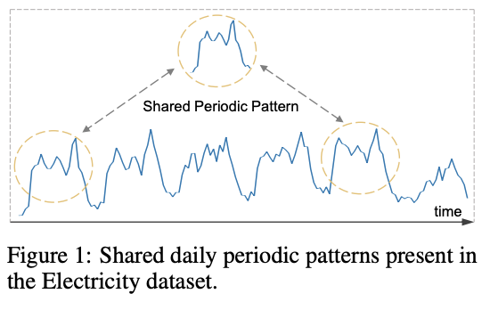
Explicit modeling of periodic patterns in the data

\(\rightarrow\) to enhance the model’s performance on LTSF tasks!

Residual Cycle Forecasting (RCF)

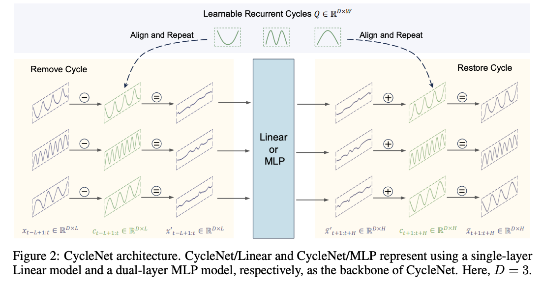
• Step 1) Learnable recurrent cycles to explicitly model the inherent periodic patterns within TS data
• Step 2) Followed by predicting the residual components of the modeled cycles.

CycleNet = RCF + Linear/MLP

2. Related Works

RCF technique

• Type of Seasonal-Trend Decomposition (STD) method.

• Key difference from existing techniques :
  • Explicit modeling of global periodic patterns within independent sequences using learnable recurrent cycles.
• Simple, computationally efficient, and yields significant improvements in prediction accuracy

Notation

• Data) TS \(X\) with \(D\) channels

• Objective) \(f: x_{t-L+1: t} \in \mathbb{R}^{L \times D} \rightarrow \bar{x}_{t+1: t+H} \in \mathbb{R}^{H \times D}\)

  • Predict future horizons \(H\) steps ahead
  • Based on past \(L\) observations

3. CycleNet

(1) Residual Cycle Forecasting

Two steps

• Step 1) Modeling the periodic patterns of sequences
  • Via learnable recurrent cycles within independent channels,
• Step 2) Predicting the residual components

Step 1) Periodic patterns modeling

( Notation: \(D\) channels & Priori cycle length \(W\) )

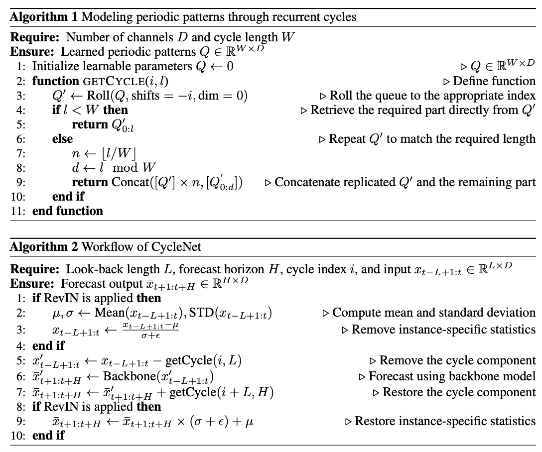
Generate learnable recurrent cycles \(Q \in \mathbb{R}^{W \times D}\)

• All initialized to zeros
• Globally shared within channels

By performing cyclic replications,

\(\rightarrow\) obtain cyclic components \(C\) of the sequence \(X\) of the same length.

Details of Cycle length \(W\)

• (1) Depends on the a priori characteristics of the dataset
• (2) Set to the maximum stable cycle within the dataset.
• (3) Easily availble
  • Considering that scenes requiring long-term predictions usually exhibit prominent, explicit cycles (e.g., electrical consumption and traffic data exhibit clear daily and weekly cycles), determining the specific cycle length is available and straightforward.
  • Cycles can be further examined through autocorrelation functions (ACF)

Step 2) Residual Forecasting

Predictions made on the residual components of the modeled cycles,

Procedure

• Step 2-1) Remove the cyclic components \(c_{t-L+1: t}\)
  • From the original input \(x_{t-L+1: t}\)
  • Obtain residual components \(x_{t-L+1: t}^{\prime}\).
• Step 2-2) Predict residual components \(\bar{x}_{t+1: t+H}^{\prime}\)
  • Using \(x_{t-L+1: t}^{\prime}\)
• Step 2-3) Add back the predicted residual components \(\bar{x}_{t+1: t+H}^{\prime}\)
  • To the cyclic components \(c_{t+1: t+H}\)
  • Obtain \(\bar{x}_{t+1: t+H}\).

Cyclic components \(C\) are virtual sequences

• derived from the cyclic replications of \(Q\),

\(\rightarrow\) Cannot directly obtain the aforementioned sub-sequences \(c_{t-L+1: t}\) and \(c_{t+1: t+H}\).

\(\therefore\) Appropriate alignments and repetitions of the recurrent cycles \(Q\) are needed!

How?

\(\begin{aligned} & c_{t-L+1: t}=[\underbrace{Q^{(t)}, \cdots, Q^{(t)}}_{\lfloor L / W\rfloor}, Q_{0: L \bmod W}^{(t)}] \\ & c_{t+1: t+H}=[\underbrace{Q^{(t+L)}, \cdots, Q^{(t+L)}}_{\lfloor H / W\rfloor}, Q_{0: H \bmod W}^{(t+L)} \end{aligned}\).

(2) Backbone

Original prediction task is transformed into…

Cyclic residual component modeling

\(\rightarrow\) Any TS model can be employed!

Opt for the most basic backbone = Linear & MLP

• CycleNet/Linear
• CycleNet/MLP

Others

• CI strategy
• RevIN
• Loss: MSE

4. Experiments

(1) Settings

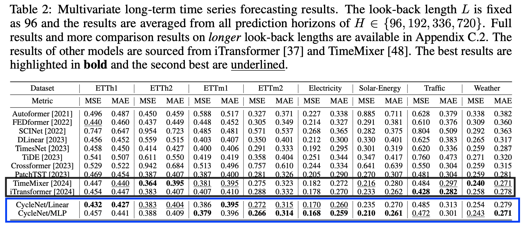
(2) LTSF

(3) Analysis

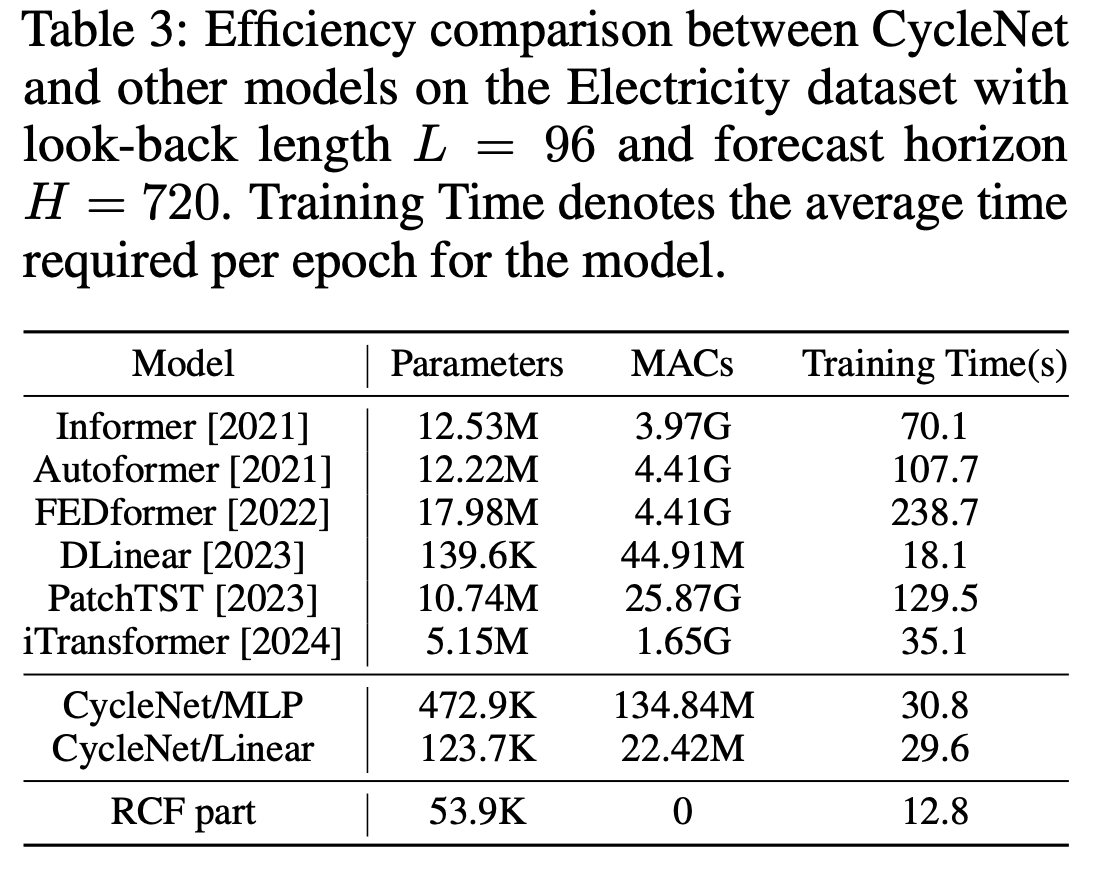
Efficiency analyiss

• Plug-and-play module
• Requires minimal overhead
  • Needing only additional W × D learnable parameters

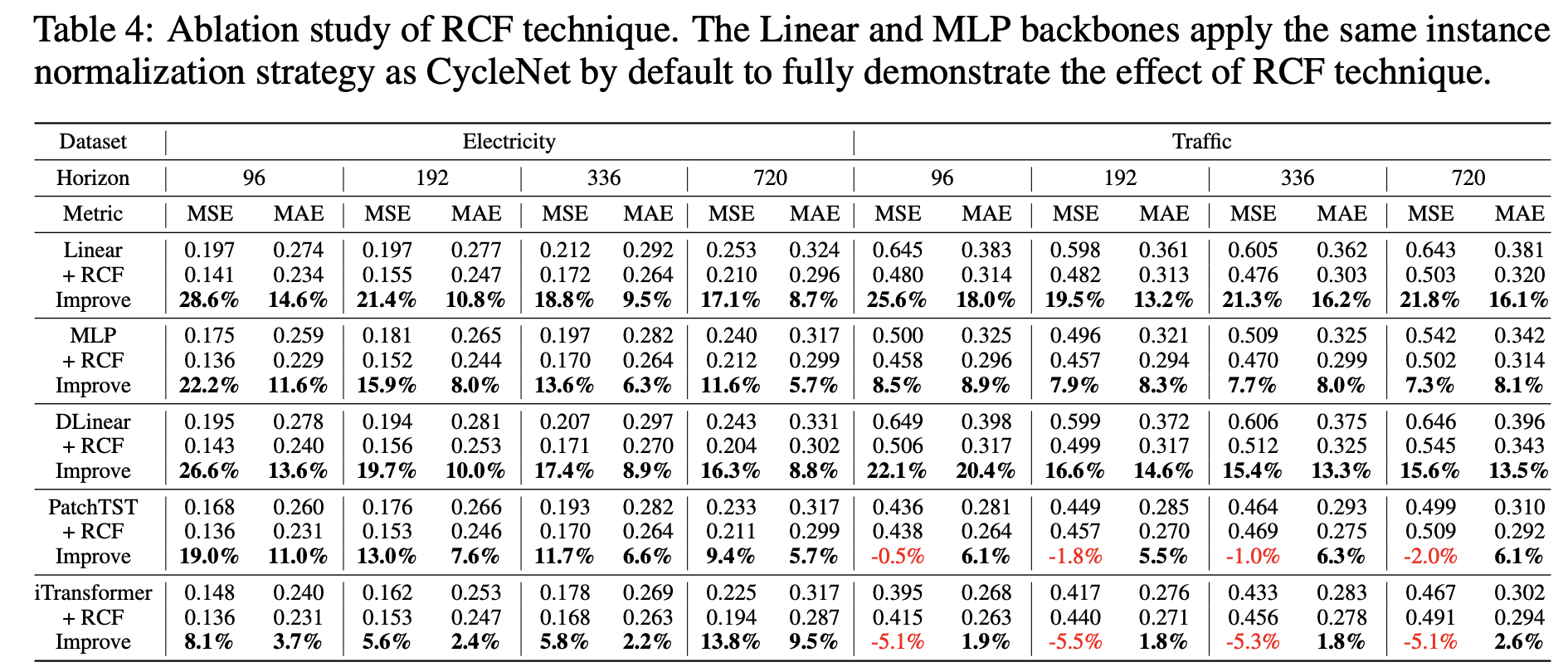
Ablation Study

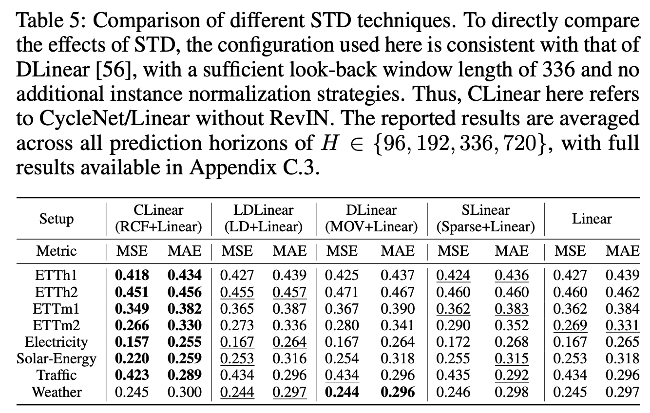
Comparison of different STD techniques

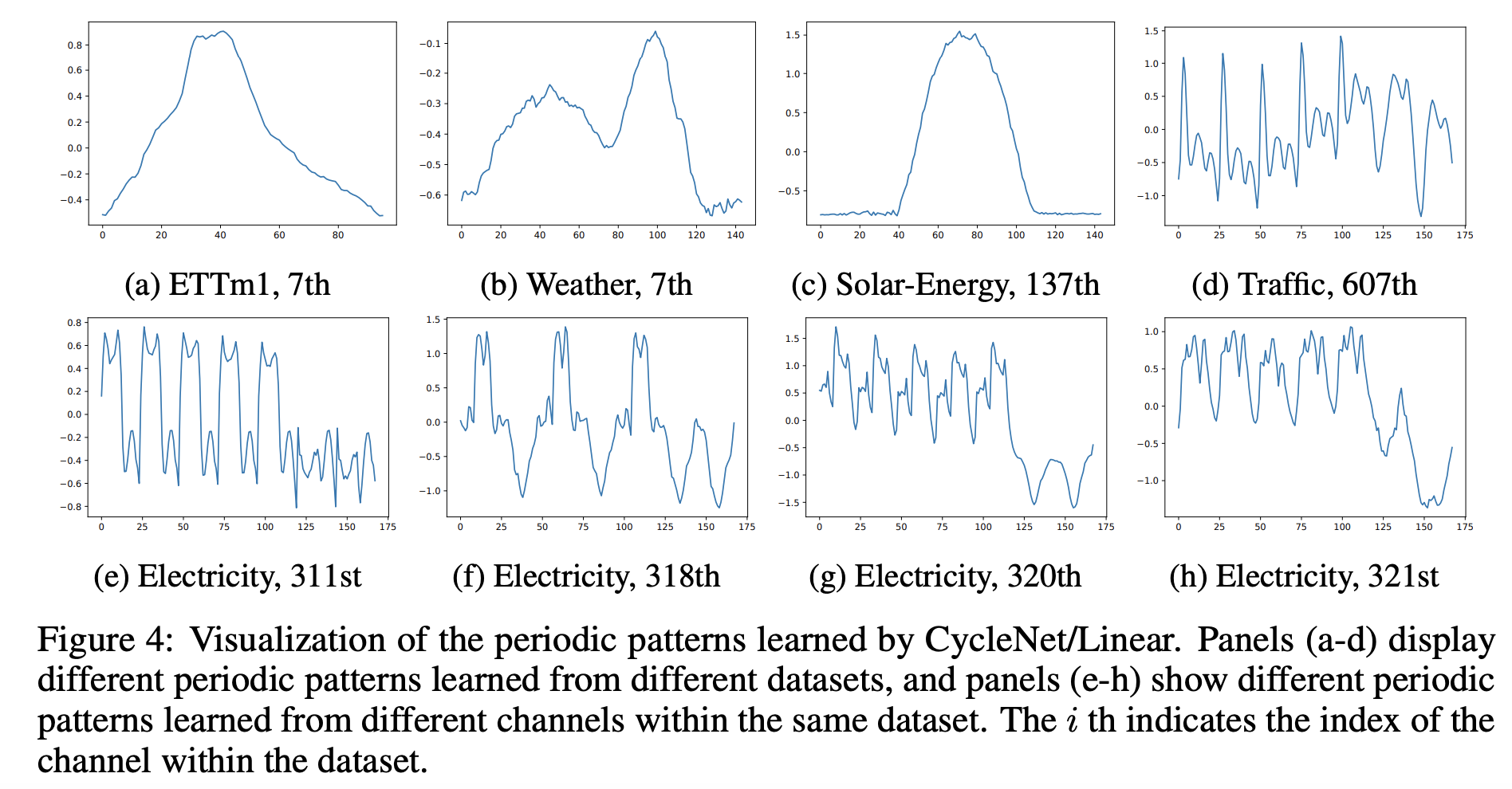
Vizualization

5. Discussion

Potential Limitation

1. Unstable cycle length
   • Unsuitable for datasets where the cycle length (or frequency) varies over time,
   • ex) Electrocardiogram (ECG) data
2. Varying cycle lengths across channels
   • When different channels within a dataset exhibit cycles of varying lengths ( due to CI )
   • Potential solution:
     • pre-process the dataset by splitting it based on cycle lengths
     • independently model each channel as a separate dataset.
3. Impact of outliers
4. Long-range cycle modeling: T