FinTSBridge: A New Evaluation Suite for Real-World Financial Prediction with Advanced Time Series Models

https://arxiv.org/pdf/2503.06928

Abstract

Problem:

기존 TSF 모델들이 많이 발전했음에도
Financial asset pricing에 실제로 적용하는 데에는 여전히 큰 간극이 존재

Goal:

최신 TSF 모델과 Finance 예측 문제를 연결하는 체계적인 evaluation bridge를 구축

Proposal: FinTSBridge

Dataset: 3개의 real-world financial TS dataset
Models: 10개 이상의 TSF 모델
Metrics
- (기존) MSE, MAE
- (제안) msIC, msIR
  - Finance 예측에서 중요한 time series correlation을 평가하기 위해

1. Introduction

(1) Problem Setting

최근 TSF 모델은 크게 발전했으나, 이를 financial asset pricing에 실제로 적용하는 데에는 여전히 큰 간극이 존재
Limitations of Existing Benchmarks
- 기존 TS benchmark는 stationarity, periodicity가 강한 데이터(electricity, traffic)에 편중
- (1) Dataset 한계점: 기존 financial dataset은
  - Daily resolution → intraday dynamics 소실
  - Limited variables → derivatives, multi-scale interaction 미반영
- (2) Metric 한계점: MSE, MAE 중심 평가는
  - Point-wise accuracy만 측정
  - temporal correlation 및 market trend alignment를 반영하지 못함
- 단순 last-value predictor도 MSE는 양호하나 → 실제 trading 관점에서는 무의미함

(2) Motivation

Financial TS에서는

(1) 예측 정확도
(2) time-series correlation
(3) economic utility

를 함께 평가하는 framework가 필요

(3) Proposed Framework: FinTSBridge

최신 TS 모델과 real-world financial prediction을 연결하는 종합 evaluation suite

Key Components

Financial-specific preprocessing
- stationarity를 강화하면서
- 변수 간 관계(inter-relationships)는 유지
Modeling stage
- 다양한 AI-based TS forecasting 모델 적용
Task design
- Multi-perspective forecasting tasks 설계
Evaluation
- 기존 metric(MSE, MAE)
- 신규 metric(msIC, msIR)
- financial metric 기반 strategy simulation

(4) Goal

단순 예측 성능을 넘어, investment decision support 관점에서 TS 모델의 실질적 활용 가능성과 robustness를 평가

기존 Financial TS 예측 연구

주로 single-step forecasting
- Next-step price prediction
- Price movement (up/down) prediction

최근 연구 흐름

Multi-horizon / multi-step forecasting으로 전환
sequence-to-sequence models 활용
- 미래 여러 시점의 trajectory를 한 번에 예측
- exchange time series의 장기 temporal dynamics 포착 목적

Cutting-edge TS models와 financial tasks 사이의 bridge 필요성 제기!

(2) The Predictability of Asset Prices

Quantitative hedge funds

Historical data에서 predictive signals을 지속적으로 발굴
Changing market environment에서도 excess return 달성

Efficient Market Hypothesis (EMH)에 대한 재해석

일부 연구:
- 시장이 semi-strong 또는 strong-form efficiency를 항상 만족하지 않는다고 주장
실제 시장:
- weak-form과 semi-strong efficiency 사이에 위치하는 경우가 많음
경험적 근거
- Momentum effect
  - 과거에 성과가 좋았던 자산이 미래에도 지속될 가능성
  - Weak-form EMH에 대한 반례
- Multi-factor models
  - asset pricing anomalies를 설명
  - 시장 효율성이 제한적임을 간접적으로 시사

기술 발전의 영향

Data processing capability의 비약적 향상
과거에는 불가능했던
- Large-scale data
- Complex non-linear patterns
을 활용한 predictive models 등장

Summary

Finance 시장은 완전 효율적이지 않으며
적절한 데이터, 모델, 평가 프레임워크 하에서는 asset price predictability가 실질적으로 존재!

3. Dataset Curation

기존 TS benchmark의 한계?

Long-term TS forecasting 연구: Electricity, weather, traffic, exchange rate 중심의 8개 mainstream dataset에 집중
Financial TS: Non-stationary, non-periodic 특성으로 인해 종종 제외되거나 ILI dataset으로 대체됨

그 결과: SOTA TS models는

Controlled dataset에서는 성능이 높지만
Real-world financial TS의 복잡성에 대한 robustness 부족

핵심 문제의식: 실제 Finance 문제를 반영하는

데이터 복잡성
비정상성
다양한 frequency

를 포함한 financial-specific dataset 필요!

(1) Data Sources

FinTSBridge는 3개의 Finance TS dataset을 구축

서로 다른 Finance sub-domain을 대표

a) GSMI

Global stock market indices
20개 주요 지수
daily frequency
기간: 2005–2024 (약 20년)
변수: price, trading volume

b) OPTION

Chinese CSI 300ETF options
call / put option의 risk-related variables
derivative market 특성 반영

c) BTCF

Bitcoin spot + perpetual futures
hourly frequency
spot–contract lag 분석
long–short trading strategy 평가에 적합

Contribution

Frequency, asset type, market structure가 다른 TS를 포괄
기존 benchmark 대비 현실 Finance 환경에 근접

(2) Data Preprocessing Methods

문제 배경: Finance TS는

변수 간 scale 차이가 큼
통일된 preprocessing 방식이 존재하지 않음

\(\rightarrow\) Task-specific preprocessing 필요

a) Log-return 기반 가격 변환 (GSMI, BTCF)

Notation

Close price series 정의
- \(P^c_{0,t} = \{p^c_0, p^c_1, \dots, p^c_t\}\).
Price change ratio
- \(R^c_i = \frac{p^c_i}{p^c_{i-1}}\).
Log transformation
- \(\ln\left(\frac{P^c_{0,t}}{p^c_0}\right) = \{0, \ln(R^c_1), \dots, \ln(R^c_t)\}\).

의미

Log price는 cumulative sum of log-returns
이전 시점 변화에만 의존 → additivity property
Non-stationarity 완화

b) High price 변환 및 관계 유지

Notation

High price series
- \(P^h_{0,t} = \{p^h_0, p^h_1, \dots, p^h_t\}\).
Relative change to last close
- \(R^h_i = \frac{p^h_i}{p^c_{i-1}}\).
Log transformation
- \(\ln\left(\frac{P^h_{0,t}}{p^c_0}\right) = \{0, \ln(R^h_1), \dots, \ln(R^h_t)\}\).

Close–high 관계

\(\Delta(P^h, P^c) = \ln\left(\frac{P^h_{0,t}}{p^c_0}\right) - \ln\left(\frac{P^c_{0,t}}{p^c_0}\right) = \{\ln(\tfrac{R^h_i}{R^c_i})\}\).

장점

OHLC 간 상대적 관계 보존
각 시점의 price structure 유지

c) Baseline anchoring

Notation

최종 가격 TS
- \(Z_{0,t} = \ln\left(\frac{P_{0,t}}{p^c_0}\right) + 100\).
목적
- Cumulative log 값의 음수 방지
- 모델 학습 안정성 향상

d) Trading volume

Notation

Volume series
- \(V_{0,t} = \{v_0, v_1, \dots, v_t\}\).
log transform
- \(Z^v_{0,t} = \ln(V_{0,t} + 1)\).

목적

Zero volume로 인한 log 오류 방지
scale 안정화

(3) Visualization of Preprocessing

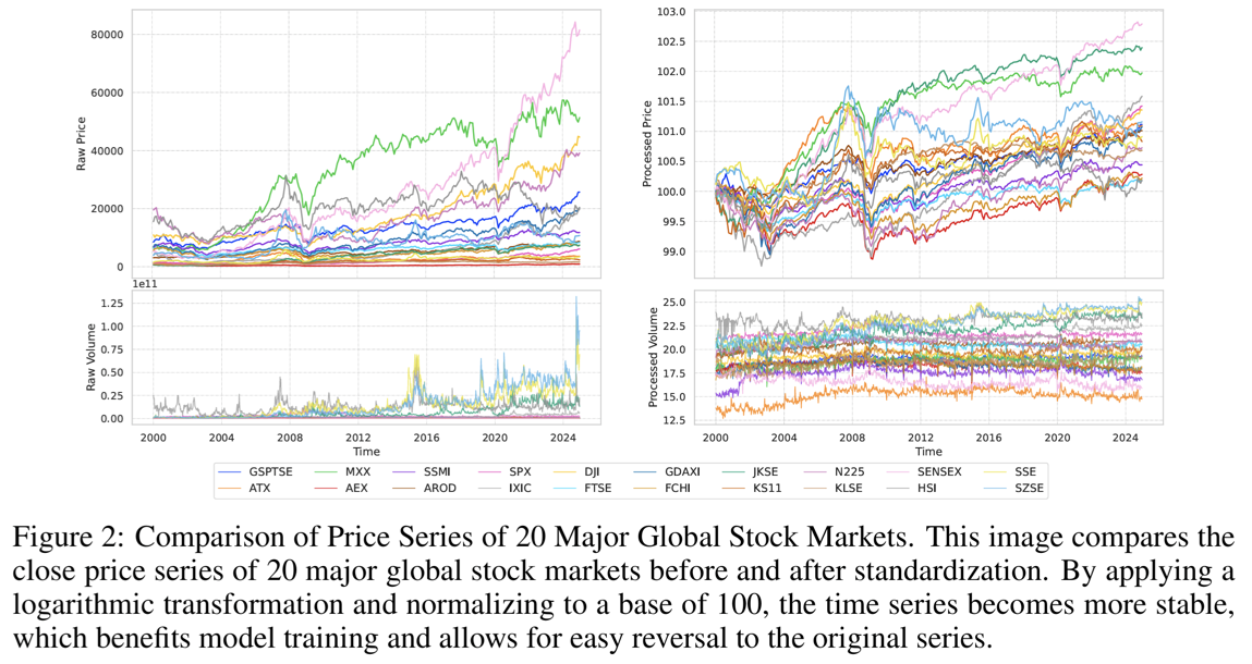
목적: 제안한 preprocessing이

(1) scale 정렬
(2) 변수 간 상대적 구조 보존

을 실제 데이터에서 어떻게 달성하는지 시각적으로 검증

**[LEFT] Preprocessing 이전**

Closing price
- 지수별 변동 폭과 절대 크기가 크게 다름
- Cross-sectional 비교가 어려움
Trading volume
- Temporal fluctuation이 매우 불안정
- 지수 간 volume 비교가 거의 불가능

[Right] Preprocessing 이후

Price & volume 모두
- 동일한 magnitude range로 정렬
- Price series는 공통 초기 baseline에 anchor

효과

Cumulative change 비교 가능
지수 간, 변수 간 일관된 비교 가능성 확보

4. New Evaluation Metrics

(1) 문제의식

기존 TS forecasting 평가

주로 MSE, MAE 같은 error-based metric에 의존

Finance TS

단순한 Naive model (last value prediction)도 낮은 MSE 달성 가능
실제 시장 trend, correlation을 거의 포착하지 못함

결론

Finance TS에서는 prediction error + correlation metric이 함께 필요

(2) 기존 Correlation metric의 한계

Information Coefficient (IC), Information Ratio (IR)

single-step
univariate

\(\rightarrow\) Multi-step, multivariate forecasting 성능을 평가하기에는 부적합

(3) Proposal

두 개의 metric 제안

msIC (multi-step IC)
msIR (multi-step IR)

목적: multi-step, multivariate TS 예측에서, 아래의 두 가지를 동시에 평가

Temporal correlation
Stability

a) msIC (Multi-step Information Coefficient)

Notation

Input: \(X \in \mathbb{R}^{B \times L \times C}\)
- \(B\): batch size
- \(L\): input length
- \(C\): number of variables
Prediction: \(\hat{Y} = f(X; \theta), \quad Y, \hat{Y} \in \mathbb{R}^{B \times F \times C}\)
- \(F\): forecast horizon

msIC 정의

(각 sample \(i\), 변수 \(j\)에 대해) Prediction horizon F에 대한 rank correlation
- \(\rho_{Y_{i,j}, \hat{Y}_{i,j}} = \frac{\text{Cov}(Y_{i,j}, \hat{Y}_{i,j})} {\sigma_{Y_{i,j}} \, \sigma_{\hat{Y}_{i,j}}} \tag{14}\).
msIC 계산
- \(\text{msIC} = \frac{1}{B \times C} \sum_{i=1}^{B} \sum_{j=1}^{C} \rho_{Y_{i,j}, \hat{Y}_{i,j}} \tag{15}\).

의미

Multi-step TS 전반에서 true TS와 predicted TS 간 temporal correlation을 직접 측정
(Error-based metric에서는 못잡아내는) trend consistency를 평가

b) msIR (Multi-step Information Ratio)

문제

msIC는 평균 correlation만 측정
sample 간 correlation stability는 반영하지 못함

msIR 정의

Sample-level msIC
- \(\text{msIC}_i = \frac{1}{C} \sum_{j=1}^{C} \rho_{Y_{i,j}, \hat{Y}_{i,j}} \tag{16}\).
msIC sequence
- \(\{\text{msIC}_1, \dots, \text{msIC}_B\}\).
- chronological order 유지
msIR 정의
- \(\text{msIR} = \frac{\text{msIC}} {\sqrt{ \frac{1}{B} \sum_{i=1}^{B} (\text{msIC}_i - \text{msIC})^2 }} \tag{18}\).
- numerator
  - 평균적인 effective correlation
- denominator
  - correlation의 temporal variability (noise)

의미

높은 msIR
- 높은 correlation
- sample 간 안정적 성능
낮은 msIR
- 일부 구간만 잘 맞고
- 전반적 신뢰도 낮음

(4) Summary

msIC는 “얼마나 잘 맞추는가”를 correlation 관점에서,
msIR는 “그 성능이 얼마나 안정적인가”를 함께 평가하는 Finance TS 특화 metric

def msIC(Y, Y_hat):
    B, F, C = Y.shape
    rhos = []

    for i in range(B):
        for j in range(C):
            y = Y[i, :, j]
            y_hat = Y_hat[i, :, j]
            rho = np.corrcoef(y, y_hat)[0, 1]
            rhos.append(rho)

    return np.mean(rhos)

def msIR(Y, Y_hat):
    B, F, C = Y.shape
    msic_per_sample = []

    for i in range(B):
        rhos = []
        for j in range(C):
            y = Y[i, :, j]
            y_hat = Y_hat[i, :, j]
            rhos.append(np.corrcoef(y, y_hat)[0, 1])
        msic_per_sample.append(np.mean(rhos))

    msic_per_sample = np.array(msic_per_sample)
    return msic_per_sample.mean() / msic_per_sample.std()

5. Experiments

(1) M2M Forecasting

Setup

Financial TS의 non-stationarity와 low signal-to-noise ratio를 고려한 실험 설계
3개 dataset × 16개 TS model 평가
Forecasting horizon
- \(H \in \{5, 21, 63, 126\}\).
Evaluation metrics
- Error-based: MSE, MAE
- Correlation-based: msIC, msIR

Results

모든 dataset·metric에서 절대적으로 우수한 단일 모델은 존재하지 않음
[1] PSformer, TimeMixer, TiDE, PatchTST
- 대부분 task에서 안정적인 성능
- PSformer가 12개 중 8개 setting에서 최고 성능
[2] Transformer, FEDformer
- Error metric에서는 열세
- 일부 dataset에서 correlation metric(msIC/msIR) 기준 경쟁력 존재
[3] Naive model
- Predictive correlation은 거의 없음
- 그럼에도 MSE/MAE는 매우 낮아, 일부 SOTA 모델보다 우수
- Financial TS의 non-stationary 특성에서 흔히 관찰되는 현상

(2) M2U Forecasting

Setup

다변량 입력을 활용한 single target forecasting
단순 예측 성능 평가뿐 아니라
- Timing trading
- Long-short trading
등 실제 Finance application 기반 investment strategy 성능 평가 포함

Results

Error metrics (MSE, MAE)
- Naive model이 대부분 경우에서 가장 낮은 loss
- PSformer, PatchTST, DLinear도 안정적인 성능
- GSMI, BTCF에서는 Naive가 최저 error
  - Price TS의 예측 난이도와 직결

Correlation metrics (msIC, msIR)

PSformer, Stationary, DLinear가 상대적으로 우수
PSformer는 12개 지표 중 9개에서 1–2위
Strategy evaluation
- Figure 7: GSMI 시장 타이밍 성능 시각화
- Table 2: 전략 수익률 및 통계 지표 비교
단순 예측 성능을 넘어 financial usability 관점에서 모델 차이를 명확히 보여줌

(3) M2P Forecasting

Setup

전체 변수 중 일부 변수만 예측하는 현실적 scenario
GSMI dataset에서
- 20개 글로벌 index의 closing price만 target으로 설정
예측 결과를 활용한 portfolio selection strategy
- 동시에 보유하는 index 개수 변화에 따른 backtest 수행

Results

Error metrics
- Naive, PatchTST가 상대적으로 우수
Correlation metrics
- PSformer, Informer가 더 강한 성능
Portfolio backtest
- 어떤 모델도 모든 holding size에서 일관된 최고 수익률은 아님
- 대부분 모델이
  - 20개 index 평균 수익률보다 높은 cumulative return 달성
  - 보유 index 수가 줄어들수록 이 경향이 더 뚜렷

(4) Summary

Financial TS에서는 error metric만으로는 모델을 평가할 수 없음
Correlation-based metric(msIC, msIR)과 strategy-level evaluation이 필수
PSformer는 전반적으로 가장 일관된 강자
Naive model의 강한 error 성능은

→ Finance TS 평가의 함정을 명확히 보여주는 사례

6. Conclusion

Advanced TSF models & Practical financial applications 간의 간극을 연결
Specialized financial datasets를 구축
- global indices, derivatives, cryptocurrency markets를 포괄
New metric 제안
- msIC와 msIR
- Multi-step forecasting에서의 temporal correlation을 정량화함

Twitter Facebook LinkedIn

AAA (All About AI)

Seunghan Lee

FinTSBridge: A New Evaluation Suite for Real-World Financial Prediction with Advanced Time Series Models

Abstract

1. Introduction

(1) Problem Setting

(2) Motivation

(3) Proposed Framework: FinTSBridge

(4) Goal

(2) The Predictability of Asset Prices

3. Dataset Curation

(1) Data Sources

a) GSMI

b) OPTION

c) BTCF

(2) Data Preprocessing Methods

a) Log-return 기반 가격 변환 (GSMI, BTCF)

b) High price 변환 및 관계 유지

c) Baseline anchoring

d) Trading volume

(3) Visualization of Preprocessing

4. New Evaluation Metrics

(1) 문제의식

(2) 기존 Correlation metric의 한계

(3) Proposal

a) msIC (Multi-step Information Coefficient)

b) msIR (Multi-step Information Ratio)

(4) Summary

5. Experiments

(1) M2M Forecasting

(2) M2U Forecasting

(3) M2P Forecasting

(4) Summary

6. Conclusion

You May Also Enjoy

AAA (All About AI)

Seunghan Lee

FinTSBridge: A New Evaluation Suite for Real-World Financial Prediction with Advanced Time Series Models

Abstract

1. Introduction

(1) Problem Setting

(2) Motivation

(3) Proposed Framework: FinTSBridge

(4) Goal

2. Related Works

(1) Financial Task-Related Studies

(2) The Predictability of Asset Prices

3. Dataset Curation

(1) Data Sources

a) GSMI

b) OPTION

c) BTCF

(2) Data Preprocessing Methods

a) Log-return 기반 가격 변환 (GSMI, BTCF)

b) High price 변환 및 관계 유지

c) Baseline anchoring

d) Trading volume

(3) Visualization of Preprocessing

4. New Evaluation Metrics

(1) 문제의식

(2) 기존 Correlation metric의 한계

(3) Proposal

a) msIC (Multi-step Information Coefficient)

b) msIR (Multi-step Information Ratio)

(4) Summary

5. Experiments

(1) M2M Forecasting

(2) M2U Forecasting

(3) M2P Forecasting

(4) Summary

6. Conclusion

You May Also Enjoy