75.Variational Inference for Dirichlet Process Mixture

Variational Inference for Dirichlet Process Mixture (2006)

Abstract

Dirichlet Process (DP) : cornerstone of non-parametric Bayesian statistics

Present a VI algorithm for DP mixtures

1. Introduction

Basic Idea of VI : into “optimization” problem

VI depends on a number of free parameters ( = variational parameters )

MCMC

• much wider application
• development for MCMC for non-parametric models ( ex. Dirichlet process )

Dirichlet Process ( DP )

• measured by…
  • 1) base distn \(G_0\)
  • 2) scaling parameter \(\alpha\)

• step 1) draw a random measure \(G\) from DP

  • \(G \mid\left\{G_{0}, \alpha\right\} \sim \operatorname{DP}\left(G_{0}, \alpha\right)\).

  step 2) draw \(N\) r.v. \(\eta_n\) from \(G\)

  • \(\eta_{n} \sim G, \quad n \in\{1, \ldots, N\}\).
• Marginalize out \(G\) …. then joint distn \(\{ \eta_1, ..., \eta-N\}\) follows Polya urn scheme

Dirichlet Process Mixture Model ( DPMM )

• adds a level to the hierarchy
• unbounded number of mixture components

Given a sample (=\(\left\{x_{1}, \ldots, x_{N}\right\}\)) from DP mixture …

• goal : compute the predictive density

  \(p\left(x \mid x_{1}, \ldots, x_{N}, \alpha, G_{0}\right)=\int p(x \mid \eta) p\left(\eta \mid x_{1}, \ldots, x_{N}, \alpha, G_{0}\right) d \eta\).

This paper presents VI for DP mixtures, based on stick-breaking representation of the underlying DP

• posterior distn \(p\)

• variational distribution \(q\)

  \(\rightarrow\) use stick-breaking representation for \(q\)

2. DPMM

Notation

• \(\eta\) : continuous r.v

• \(G_0\) : base distn for \(\eta\)

• \(\alpha\) : scale parameter

• \(k\) partitions : \(\left\{B_{1}, \ldots, B_{k}\right\}\)

  \(\rightarrow\) \(G\) is distributed according to a DP

  \(\left(G\left(B_{1}\right), G\left(B_{2}\right), \ldots, G\left(B_{k}\right)\right) \sim \operatorname{Dir}\left(\alpha G_{0}\left(B_{1}\right), \alpha G_{0}\left(B_{2}\right), \ldots, \alpha G_{0}\left(B_{k}\right)\right)\).

Integrate out \(G\) & condition on \(n-1\) draws…

• \(p\left(\eta_n \mid \eta_{1}, \ldots, \eta_{n-1}\right) \propto \alpha G_{0}(\cdot)+\sum_{i=1}^{n-1} \delta_{\eta_{i}}(\cdot)\).

• Polya Urn Scheme :

  \(\eta_{n}=\left\{\begin{aligned} \eta_{i}^{*} & \text { with prob. } \frac{\mid \left\{j: c_{j}=i\right\} \mid}{n-1+\alpha} \\ \eta, \eta \sim G_{0} & \text { with prob. } \frac{\alpha}{n-1+\alpha} \end{aligned}\right.\).

  where \(\mid \left\{j: c_{j}=i\right\} \mid\) is the number of times the value \(\eta_{i}^{*}\) occurs in \(\left\{\eta_{1}, \ldots, \eta_{n-1}\right\}\).

in DPMM, DPis used as a non-parametric prior

\(\begin{aligned} G \mid\left\{\alpha, G_{0}\right\} & \sim \operatorname{DP}\left(\alpha, G_{0}\right) \\ \eta_{n} \mid G & \sim G \\ X_{n} \mid \eta_{n} & \sim p\left(x_{n} \mid \eta_{n}\right) \end{aligned}\).

• ex) \(\eta_7 = (0.2,0.3,0.5)\)

• interpretation : flexible mixture model,

  in which the number of components is random & grows as new data are observed

Stick-breaking Construction

1) \(V_{i} \sim \operatorname{Beta}(1, \alpha)\).

• \(\pi_{i}(\mathbf{v})=v_{i} \prod_{j=1}^{i-1}\left(1-v_{j}\right)\).
• ex) \(\pi_{7}(\mathbf{v})=0.3\) ( mixing proportion )

2) \(\eta_{i}^{*} \sim G_{0}\).

• ex) \(\eta_7^* = 4\) & \(\delta_{\eta_{7}^{*}}=(0,0,0,1,.....0)\)

Thus… \(G=\sum_{i=1}^{\infty} \pi_{i}(\mathbf{v}) \delta_{\eta_{i}^{*}}\).

This representation of DP makes clear that “\(G\) is discrete”

• support of \(G\) : countably infinite set of atms

In DP mixture…

• \(\pi_{\mathbf{v}}\) : comprises of infinite vector of mixing proportions
• \(\left\{\eta_{1}^{*}, \eta_{2}^{*}, \ldots\right\}\) : atoms representing mixture components

[ Algorithm ]

1. Draw \(V_{i} \mid \alpha \sim \operatorname{Beta}(1, \alpha), \quad i=\{1,2, \ldots\}\)
2. Draw \(\eta_{i}^{*} \mid G_{0} \sim G_{0}, \quad i=\{1,2, \ldots\}\)
3. For the \(n\) th data point: (a) Draw \(Z_{n} \mid\left\{v_{1}, v_{2}, \ldots\right\} \sim \operatorname{Mult}(\pi(\mathbf{v}))\). (b) Draw \(X_{n} \mid z_{n} \sim p\left(x_{n} \mid \eta_{z_{n}}^{*}\right)\).

In this paper, restrict DP mixtures, for which the data are drawn from an exponential family

• \(p\left(x_{n} \mid z_{n}, \eta_{1}^{*}, \eta_{2}^{*}, \ldots\right)=\prod_{i=1}^{\infty}\left(h\left(x_{n}\right) \exp \left\{\eta_{i}^{* T} x_{n}-a\left(\eta_{i}^{*}\right)\right\}\right)^{\mathbf{1}\left[z_{n}=i\right]}\).

• base distn )

  \(p\left(\eta^{*} \mid \lambda\right)=h\left(\eta^{*}\right) \exp \left\{\lambda_{1}^{T} \eta^{*}+\lambda_{2}\left(-a\left(\eta^{*}\right)\right)-a(\lambda)\right\}\).

3. Variational Inference for DP mixtures

no direct way to compute posterior, under DP mixture

use Variational Inference

notation

• \(\theta\) : hyperparameters
• \(\mathbf{W}=\left\{W_{1}, \ldots, W_{M}\right\}\) : latent variables
• \(\mathrm{x}=\left\{x_{1}, \ldots, x_{N}\right\}\) : observations

posterior distribution of latent variables :

• \(p(\mathbf{w} \mid \mathbf{x}, \theta)=\exp \{\log p(\mathbf{x}, \mathbf{w} \mid \theta)-\log p(\mathbf{x} \mid \theta)\}\).

Gibbs sampling

• \(p\left(w_{i} \mid \mathbf{w}_{-i}, \mathbf{x}, \theta\right)=\exp \left\{\log p(\mathbf{w}, \mathbf{x} \mid \theta)-\log p\left(\mathbf{w}_{-i}, \mathbf{x} \mid \theta\right)\right\}\).

Variational inference

• Minimize KL-divergence :

  \(\mathrm{D}\left(q_{\nu}(\mathbf{w}) \mid p(\mathbf{w} \mid \mathbf{x}, \theta)\right)=\mathrm{E}_{q}\left[\log q_{\nu}(\mathbf{W})\right]-\mathrm{E}_{q}[\log p(\mathbf{W}, \mathbf{x} \mid \theta)]+\log p(\mathbf{x} \mid \theta)\).

• Maximize ELBO :

  \(\log p(\mathbf{x} \mid \theta) \geq \mathrm{E}_{q}[\log p(\mathbf{W}, \mathbf{x} \mid \theta)]-\mathrm{E}_{q}\left[\log q_{\nu}(\mathbf{W})\right]\).

3-1. MFVI in exponential families

Assume that conditional distn \(p\left(w_{i} \mid \mathbf{w}_{-i}, \mathbf{x}, \theta\right)\) is exponential family

• \(p\left(w_{i} \mid \mathbf{w}_{-i}, \mathbf{x}, \theta\right)=h\left(w_{i}\right) \exp \left\{g_{i}\left(\mathbf{w}_{-i}, \mathbf{x}, \theta\right)^{T} w_{i}-a\left(g_{i}\left(\mathbf{w}_{-i}, \mathbf{x}, \theta\right)\right)\right\}\).

Mean Field Variational Inference (MFVI)

• variational parameter \(\nu_i\)

• factorize as \(q_{\nu}(\mathbf{w})=\prod_{i=1}^{M} \exp \left\{\nu_{i}^{T} w_{i}-a\left(w_{i}\right)\right\}\).
• solution : \(\nu_{i}=\mathrm{E}_{q}\left[g_{i}\left(\mathbf{W}_{-i}, \mathbf{x}, \theta\right)\right]\).

Gibbs Sampler & MFVI

• Gibbs sampler : draw the latent variables \(w_{i}\) from the distribution \(p\left(w_{i} \mid \mathbf{w}_{-i}, \mathbf{x}, \theta\right)\)
• MFVI : \(\nu_{i}=\mathrm{E}_{q}\left[g_{i}\left(\mathbf{W}_{-i}, \mathbf{x}, \theta\right)\right]\).

3-2. DP mixtures

MFVI for DP mixtures

• based on stick-breaking representation of DP mixture
• latent variables : \(\mathbf{W}=\left\{\mathbf{V}, \boldsymbol{\eta}^{*}, \mathbf{Z}\right\}\)
  • stick length : \(\mathbf{V}\)
  • atoms : \(\eta^*\)
  • cluster assignments : \(\mathbf{Z}\)
• hyperparameters : \(\theta=\{\alpha, \lambda\}\)
  • scaling parameter : \(\alpha\)
  • parameter of conjugate base distn \(\lambda\)

ELBO :

\(\begin{aligned} \log p(\mathbf{x} \mid \alpha, \lambda) \geq & \mathrm{E}_{q}[\log p(\mathbf{V} \mid \alpha)]+\mathrm{E}_{q}\left[\log p\left(\boldsymbol{\eta}^{*} \mid \lambda\right)\right] \\ &+\sum_{n=1}^{N}\left(\mathrm{E}_{q}\left[\log p\left(Z_{n} \mid \mathbf{V}\right)\right]+\mathrm{E}_{q}\left[\log p\left(x_{n} \mid Z_{n}\right)\right]\right) \\ &-\mathrm{E}_{q}\left[\log q\left(\mathbf{V}, \eta^{*}, \mathbf{Z}\right)\right] \end{aligned}\).

MFVI : factorized family

• \(q\left(\mathbf{v}, \boldsymbol{\eta}^{*}, \mathbf{z}\right)=\prod_{t=1}^{T-1} q_{\gamma_{t}}\left(v_{t}\right) \prod_{t=1}^{T} q_{\tau_{t}}\left(\eta_{t}^{*}\right) \prod_{n=1}^{N} q_{\phi_{n}}\left(z_{n}\right)\).

  • \(q_{\gamma_{t}}\left(v_{t}\right)\) : Beta distn
  • \(q_{\tau_{t}}\left(\eta_{t}^{*}\right)\) : exponential family natural parameters \(\tau_{t}\)
  • \(q_{\phi_{n}}\left(z_{n}\right)\) : multinomial distributions

• free variational parameters :

  \(\nu=\left\{\gamma_{1}, \ldots, \gamma_{T-1}, \tau_{1}, \ldots, \tau_{T}, \phi_{1}, \ldots, \phi_{N}\right\}\).

There is a different variational parameter for each latent variable, under the variational distn

Coordinate ascent algorithm

algorithm for optimizing ELBO

all terms above, except third term involve standard computation in the exponential family

**Third Term : **

\(\begin{aligned} \mathrm{E}_{q}\left[\log p\left(Z_{n} \mid \mathbf{V}\right)\right] &=\mathrm{E}_{q}\left[\log \left(\prod_{i=1}^{\infty}\left(1-V_{i}\right)^{1\left[Z_{n}>i\right]} V_{i}^{1\left[Z_{n}=i\right]}\right)\right] \\ &=\sum_{i=1}^{\infty} q\left(z_{n}>i\right) \mathrm{E}_{q}\left[\log \left(1-V_{i}\right)\right]+q\left(z_{n}=i\right) \mathrm{E}_{q}\left[\log V_{i}\right] . \end{aligned}\).

• truncate this at \(t=T\) :

  \(\mathrm{E}_{q}\left[\log p\left(Z_{n} \mid \mathbf{V}\right)\right]=\sum_{i=1}^{T} q\left(z_{n}>i\right) \mathrm{E}_{q}\left[\log \left(1-V_{i}\right)\right]+q\left(z_{n}=i\right) \mathrm{E}_{q}\left[\log V_{i}\right]\).

  where

  • \(q\left(z_{n}=i\right) =\phi_{n, i}\).
  • \(q\left(z_{n}>i\right) =\sum_{j=i+1}^{T} \phi_{n, j}\).
  • \(\mathrm{E}_{q}\left[\log V_{i}\right] =\Psi\left(\gamma_{i, 1}\right)-\Psi\left(\gamma_{i, 1}+\gamma_{i, 2}\right)\).
  • \(\mathrm{E}_{q}\left[\log \left(1-V_{i}\right)\right] =\Psi\left(\gamma_{i, 2}\right)-\Psi\left(\gamma_{i, 1}+\gamma_{i, 2}\right)\).

Solution of coordinate-update :

• \(\nu_{i}=\mathrm{E}_{q}\left[g_{i}\left(\mathbf{W}_{-i}, \mathbf{x}, \theta\right)\right]\).

  where \(\nu=\left\{\gamma_{1}, \ldots, \gamma_{T-1}, \tau_{1}, \ldots, \tau_{T}, \phi_{1}, \ldots, \phi_{N}\right\}\)

\(\begin{aligned} \gamma_{t, 1} &=1+\sum_{n} \phi_{n, t} \\ \gamma_{t, 2} &=\alpha+\sum_{n} \sum_{j=t+1}^{T} \phi_{n, j} \\ \tau_{t, 1} &=\lambda_{1}+\sum_{n} \phi_{n, t} x_{n} \\ \tau_{t, 2} &=\lambda_{2}+\sum_{n} \phi_{n, t} \\ \phi_{n, t} & \propto \exp \left(S_{t}\right) \end{aligned}\).

• where \(S_{t}=\mathrm{E}_{q}\left[\log V_{t}\right]+\sum_{i=1}^{t-1} \mathrm{E}_{q}\left[\log \left(1-V_{i}\right)\right]+\mathrm{E}_{q}\left[\eta_{t}^{*}\right]^{T} X_{n}-\mathrm{E}_{q}\left[a\left(\eta_{t}^{*}\right)\right]\)

Iterate these above equations!

Predictive Distribution

• \(p\left(x_{N+1} \mid \mathbf{x}, \alpha, \lambda\right)=\int\left(\sum_{t=1}^{\infty} \pi_{t}(\mathbf{v}) p\left(x_{N+1} \mid \eta_{t}^{*}\right)\right) d P\left(\mathbf{v}, \boldsymbol{\eta}^{*} \mid \mathbf{x}, \lambda, \alpha\right)\).

  \(p\left(x_{N+1} \mid \mathbf{x}, \alpha, \lambda\right) \approx \sum_{t=1}^{T} \mathrm{E}_{q}\left[\pi_{t}(\mathbf{V})\right] \mathrm{E}_{q}\left[p\left(x_{N+1} \mid \eta_{t}^{*}\right)\right]\).

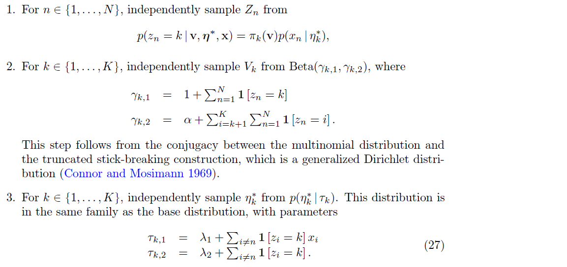
4. Gibbs Sampling

4-1. Collapsed Gibbs sampling

Markov Chain is only defined on the latent partition \(\mathbf{c}=\left\{c_{1}, \ldots, c_{N}\right\}\)

( integrate out \(G\) and \(\left\{\eta_{1}^{*}, \ldots, \eta_{\mid \mathrm{c} \mid }^{*}\right\}\) )

Assignment \(C_{n}\) can be one of \(\mid\mathbf{c}_{-n}\mid+1\) values

Exchangeability implies that \(C_{n}\) has multinomial distn :

• \(p\left(c_{n}=k \mid \mathbf{x}, \mathbf{c}_{-n}, \lambda, \alpha\right) \propto p\left(x_{n} \mid \mathbf{x}_{-n}, \mathbf{c}_{-n}, c_{n}=k, \lambda\right) p\left(c_{n}=k \mid \mathbf{c}_{-n}, \alpha\right)\).

First term : \(p\left(x_{n} \mid \mathbf{x}_{-n}, \mathbf{c}_{-n}, c_{n}=k, \lambda\right)\).

• ratio of normalizing constants of posterior distn of \(k\)th param
• \(\begin{array}{l} p\left(x_{n} \mid \mathbf{x}_{-n}, \mathbf{c}_{-n}, c_{n}=k, \lambda\right)= \frac{\exp \left\{a\left(\lambda_{1}+\sum_{m \neq n} 1\left[c_{m}=k\right] x_{m}+x_{n}, \lambda_{2}+\sum_{m \neq n} 1\left[c_{m}=k\right]+1\right)\right\}}{\exp \left\{a\left(\lambda_{1}+\sum_{m \neq n} 1\left[c_{m}=k\right] x_{m}, \lambda_{2}+\sum_{m \neq n} 1\left[c_{m}=k\right]\right)\right\}} \end{array}\).

Second term : \(p\left(c_{n}=k \mid \mathbf{c}_{-n}, \alpha\right)\).

• given by Polya urn scheme

• \(p\left(c_{n}=k \mid \mathbf{c}_{-n}\right) \propto\left\{\begin{array}{ll} \mid\left\{j: c_{-n, j}=k\right\}\mid & \text { if } k \text { is an existing cell in the partition } \\ \alpha & \text { if } k \text { is a new cell in the partition, } \end{array}\right.\).

  where \(\mid\left\{j: c_{-n, j}=k\right\}\mid\) : number of data points in the \(k\) th cell of the partition

After chain reached stationary distn, collect \(B\) samples : \(\left\{\mathbf{c}_{1}, \ldots, \mathbf{c}_{B}\right\}\).

Predictive Distribution

\(p\left(x_{N+1} \mid x_{1}, \ldots, x_{N}, \alpha, \lambda\right)=\frac{1}{B} \sum_{b=1}^{B} p\left(x_{N+1} \mid \mathbf{c}_{b}, \mathbf{x}, \alpha, \lambda\right)\).

• where \(p\left(x_{N+1} \mid \mathbf{c}_{b}, \mathbf{x}, \alpha, \lambda\right)=\sum_{k=1}^{\mid\mathbf{c}_{b}\mid+1} p\left(c_{N+1}=k \mid \mathbf{c}_{b}, \alpha\right) p\left(x_{N+1} \mid \mathbf{c}_{b}, \mathbf{x}, c_{N+1}=k, \lambda\right)\).

4-2. Blocked Gibbs sampling

Based on the stick-breaking representation

One needs to sample the infinite collection of stick lengths \(\mathbf{V}\),

before sampling the finite collection of cluster assignments \(\mathbf{Z}\)

\(\rightarrow\) solve this using truncated D (TDP)

• \(\mathbf{V_{k-1}}\) is set equal to one fore some fixed value \(K\)
• Thus, \(\pi_{i}(\mathbf{V})=0 \text { for } i \geq K\).
• converts infinite sum into finite sum

notation

• beta variables : \(\mathbf{V}=\left\{V_{1}, \ldots, V_{K-1}\right\}\).
• mixture component parameters : \(\boldsymbol{\eta}^{*}=\left\{\eta_{1}^{*}, \ldots, \eta_{K}^{*}\right\}\)
• indicator variables :\(\mathbf{Z}=\left\{Z_{1}, \ldots, Z_{N}\right\}\)

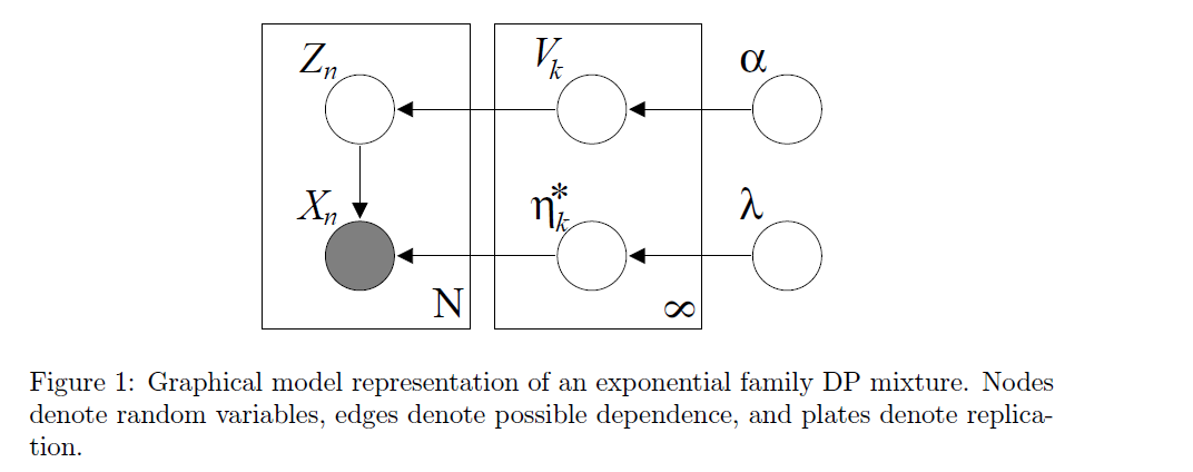
[ Blocked Gibbs : 3 steps ]

Predictive Distribution

• approximate predictive distn

• \(p\left(x_{N+1} \mid \mathbf{z}, \mathbf{x}, \alpha, \lambda\right)=\sum_{k=1}^{K} \mathrm{E}\left[\pi_{i}(\mathbf{V}) \mid \gamma_{1}, \ldots, \gamma_{k}\right] p\left(x_{N+1} \mid \tau_{k}\right)\)>

  • where \(\mathrm{E}\left[\pi_{i} \mid \gamma_{1}, \ldots, \gamma_{k}\right]\) is the expectation of the product of independent beta variables

    given in \(\pi_{i}(\mathbf{v})=v_{i} \prod_{j=1}^{i-1}\left(1-v_{j}\right)\) and \(V_{i} \sim \operatorname{Beta}(1, \alpha)\)

    
    

5. Conclusion

developed MFVI for DPMM

• faster than Gibbs sampling
• convergence time was independent of dimensionality