
Bijectors for NF
( 참고 : coursera : Probabilistic Deep Learning with Tensorflow2, Tensorflow official website )
Contents
- Bijector
- Scale bijectors and linear operator
- Transformed Distribution
- Subclassing Bijectors
- Training Bijector
import numpy as np
import pandas as pd
import matplotlib.pyplot as plt

import tensorflow as tf
import tensorflow_probability as tfp
tfd = tfp.distributions
tfb = tfp.bijectors
tfpl = tfp.layers
1. Bijector
tfb.Chain,tfb.Shift,tfb.Scale를 사용하여, 분포 \(z\)를 \(x\)로 변화시키기!
(a) make Bijector
example ) scale_n_shift Bijector를 다음과 같이 만든다.
scale=4.5
shift=7
scale_n_shift = tfb.Chain([tfb.Shift(shift),tfb.Scale(scale)])

####### 또 다른 방법 #############
scale_1 = tfb.Scale(scale)
shift_2 = tfb.Shift(shift)
scale_n_shift = shift_2(scale_1)
(b) Forward
\(z\)를 \(x\)로 transform한다 ( 다시 scaling해서 0으로 만듬을 확인할 수 있다 )
n=10000
z=normal.sample(n)

x = scale_n_shift(z)
tf.norm(x-(scale*z+shift))
<tf.Tensor: shape=(), dtype=float32, numpy=0.0>
(c) Inverse
forward & inverse를 통해원래대로 돌아옴을 확인할 수 있다
inv_x = scale_n_shift.inverse(x)
tf.norm(inv_x-z)
(d) Normalizing Flow
log_prob_x = normal.log_prob(z) - scale_n_shift.forward_log_det_jacobian(z,event_ndims=0)

# z = scale_n_shift.inverse(x) 이기 때문에, 아래와 같이 표현해도 무방하다.
log_prob_x2 = normal.log_prob(scale_n_shift.inverse(x)) + scale_n_shift.inverse_log_det_jacobian(x,event_ndims=0)
(e) example of Bijectors
다음과 같은 2개의 bijector에 대해 알아볼것이다.
- 1) Softfloor bijector
- 2) GumbelCDF bijector
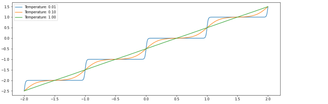
Softfloor bijector
- compute a differentiable approximation to
tf.math.floor(x) softfloor(x, t) = a * sigmoid((x - 1.) / t) + ba = 1 / (sigmoid(0.5 / t) - sigmoid(-0.5 / t))b = -sigmoid(-0.5 / t) / (sigmoid(0.5 / t) - sigmoid(-0.5 / t))
x = tf.random.normal(shape=(100,1))
sf = tfb.Softfloor(temperature=[0.2,0.1])
y = sf.forward(x)  # shape : (100,2)
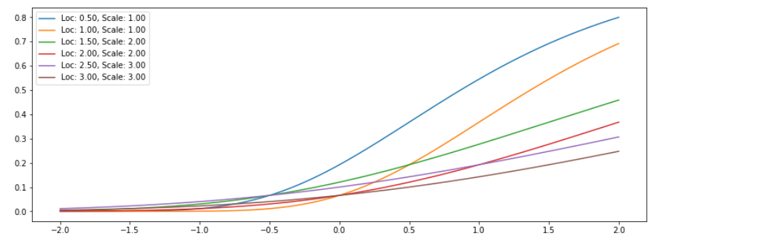
GumbelCDF bijector
- \(F(x)=e^{-e^{(-x)}}\).
exps = tfb.GumbelCDF(loc=[0.5,1.0,1.5,2.0,2.5,3],scale=[1,1,2,2,3,3])
2. Scale bijectors and linear operator
Bijector는 위의 경우처럼 1차원 데이터에만 국한되지 않는다. 보다 고차원의 Bijector도 아래와 같이 생성할 수 있다.
-
ScaleMatvec-
ScaleMatvecDiag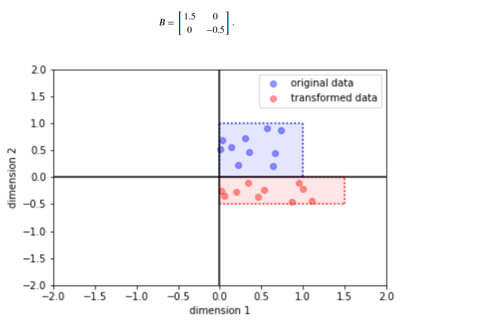
-
ScaleMatvecTriL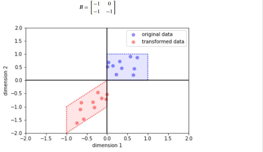
-
-
ScaleMatvecLinearOperator-
class :
LinearOperatorDiag -
class :
LinearOperatorFullMatrix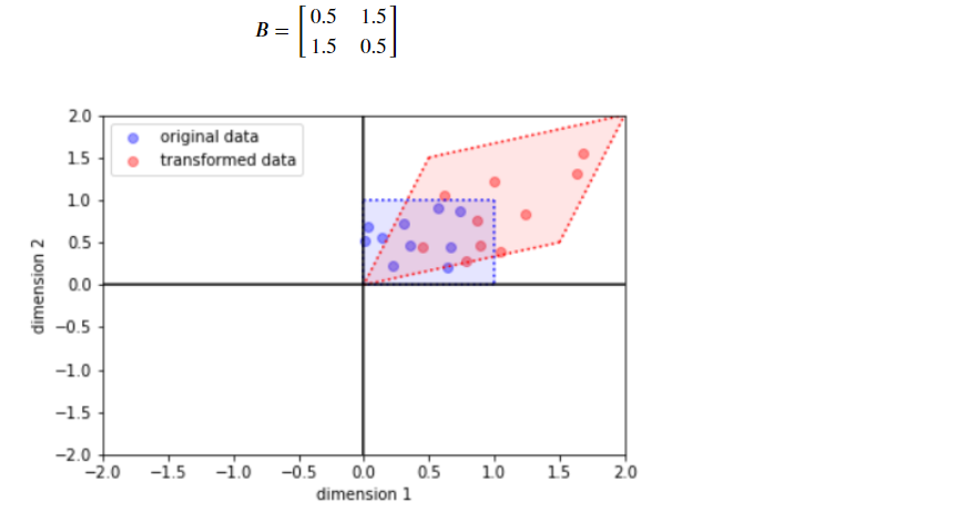
-
2-1. ScaleMatvec
(a) ScaleMatvecDiag
bijector = tfb.ScaleMatvecDiag(scale_diag=[1.5, -0.5])
y = bijector(x)
(b) ScaleMatvecTriL
bijector = tfb.ScaleMatvecTriL(scale_tril=[[-1., 0.],
                                           [-1., -1.]])
y = bijector(x)
2-2. ScaleMatvecLinearOperator
( ScaleMatvec와는 다르게, LinearOperator를 통해 scale을 먼저 생성해주고, 이를 input으로 넣어야 한다. )
(a) LinearOperatorDiag
scale = tf.linalg.LinearOperatorDiag(diag=[1.5, -0.5])
bijector = tfb.ScaleMatvecLinearOperator(scale)
y = bijector(x)
(b) LinearOperatorFullMatrix
B = [[0.5, 1.5],
     [1.5, 0.5]]
scale = tf.linalg.LinearOperatorFullMatrix(matrix=B)
bijector = tfb.ScaleMatvecLinearOperator(scale)
y = bijector(x)
3. Transformed Distribution
A=tfd.TransformedDistribution(B,C)
- A : Data distribution
- B : Base distribution
- C : Bijector
normal = tfd.Normal(loc=0.0,scale=1.0)

bijector1 = tfb.Exp()
bijector2 = tfb.ScaleMatvecTriL(scale_tril=[[1.0,0.0],[1.0,1.0]])
bijector3 = tfb.ScaleMatvecTriL(scale_tril=[[1.0,0.0],[1.0,1.0]])

log_normal = tfd.TransformedDistribution(normal,bijector1)
mvn = tfd.TransformedDistribution(normal,bijector2, event_shape=[2])
mvn2 = tfd.TransformedDistribution(normal,bijector3, batch_shape=[2],event_shape=[2])
Example
# (1) Base
normal = tfd.Normal(loc=0,scale=1)

# (2) Bijector
batch_shape=2
event_shape=4

tril = tf.random.normal((batch_shape,event_shape,event_shape))
scale_low_tri = tf.linalg.LinearOperatorLowerTriangular(tril)
scale_lin_op = tfb.ScaleMatvecLinearOperator(scale_low_tri)

# (3) Result
mvn = tfd.TransformedDistribution(normal,scale_lin_op,
                                 batch_shape=[batch_shape],event_shape=[event_shape])
Transformed 된 분포에서의 sample
n = 100
y = mvn.sample(sample_shape=(n,)) # shape : (100,batch_shape,event_shape)
4. Subclassing Bijectors
다음과 같은 Cubic Bijector를 만들어보자.
\(y=(ax+b)^3\). ( code : tf.squeeze(tf.pow(self.a*x + self.b,3)) )
다음의 함수는 반드시 들어가야 한다.
- _forward
- _inverse
- _forward_log_det_jacobian
class Cubic(tfb.Bijector):
    def __init__(self, a, b, validate_args=False, name='Cubic'):
        self.a = tf.cast(a, tf.float32)
        self.b = tf.cast(b, tf.float32)
        if validate_args:
            assert tf.reduce_mean(tf.cast(tf.math.greater_equal(tf.abs(self.a), 1e-5), tf.float32)) == 1.0
            assert tf.reduce_mean(tf.cast(tf.math.greater_equal(tf.abs(self.b), 1e-5), tf.float32)) == 1.0
        super(Cubic, self).__init__(
            validate_args=validate_args, forward_min_event_ndims=0, name=name)

    def _forward(self,x):
        x = tf.cast(x,tf.float32)
        return tf.squeeze(tf.pow(self.a*x + self.b,3))

    def _inverse(self,y):
        y = tf.cast(y,tf.float32)
        return (tf.math.sign(y)*tf.pow(tf.abs(y),1/3)-self.b)/self.a

    def _forward_log_det_jacobian(self,x):
        x = tf.cast(x,tf.float32)
        return tf.math.log(3.*tf.abs(self.a))+2.*tf.math.log(tf.abs(self.a*x+self.b))
# example
cubic = Cubic([1.0,-2.0],[-1.0,0.4],validate_args=True)
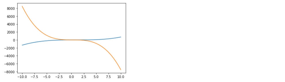
4-1. Forward
cubic.forward(x) ( 혹은 그냥 cubic(x) )
x = np.linspace(-10,10,500).reshape(-1,1)
plt.plot(x,cubic.forward(x))
plt.show()
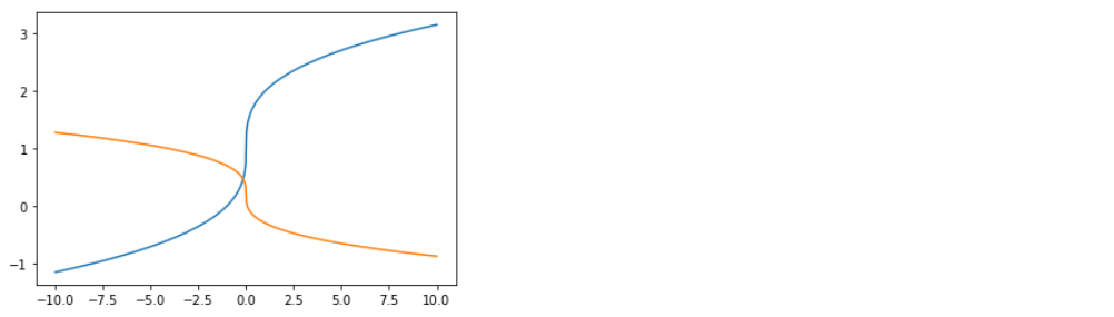
4-2. Inverse
cubic.inverse(x) ( 혹은 그냥 cubic(x) )
plt.plot(x,cubic.inverse(x))
plt.show()
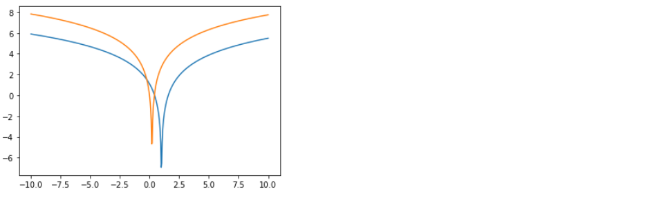
4-3. Log determinant
cubic.forward_log_det_jacobian(x,event_ndims)
plt.plot(x,cubic.forward_log_det_jacobian(x,event_ndims=0))
plt.show()
4-4. Transformed Distribution
위에서 만든 cubic bijector를 사용해서 base distribution (normal)을 변화시킨다
# (1) Base distn
normal = tfd.Normal(loc=0.,scale=1.)

# (2) Bijector
cubic = Cubic([1.0,-2.0],[-1.0,0.4],validate_args=True)

# (3) Transformed distn
cubed_normal= tfd.TransformedDistribution(normal,cubic,event_shape=[2])
tfb.Invert()를 통해 bijector의 inverse를 구할 수 있다.
( tfd.TransformedDistribution를 또 한번 사용할 필요가 없다 )
# (1) Base distn
normal = tfd.Normal(loc=0.,scale=1.)

# (2) Bijector
cubic = Cubic([1.0,-2.0],[-1.0,0.4],validate_args=True)
inverse_cubic = tfb.Invert(cubic)

# (3) Transformed distn
inv_cubed_normal= inverse_cubic(normal,event_shape=[2])
5. Training Bijector
Gaussian Mixture를 사례로, Bijector를 학습시켜볼 것이다.
( 즉, 얼마나 scaling되고 shift되는지 그 “정도”를 학습시키는 것이다 )
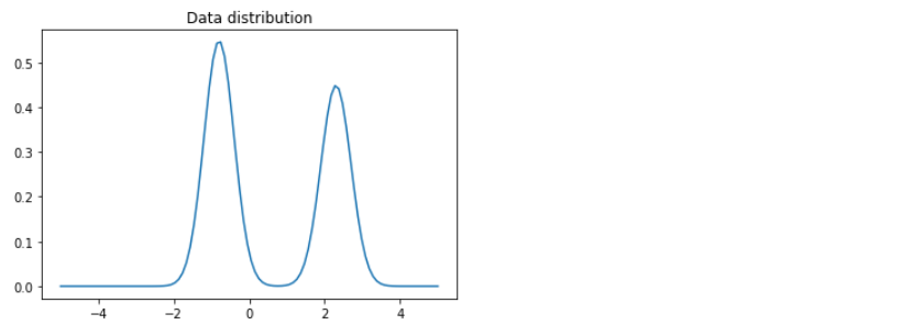
5-1. 가상의 정답 분포 생성
GMM with 2 components
- \(\mu_1=2.3\) , \(\sigma_1 = 0.4\), ……\(w_1 = 0.45\)
- \(\mu_2=-0.8\) , \(\sigma_2 = 0.4\) …….\(w_2 = 0.55\)
probs = [0.45,0.55]

mix_gauss = tfd.Mixture(
    cat=tfd.Categorical(probs=probs),
    components=[
        tfd.Normal(loc=2.3,scale=0.4),
        tfd.Normal(loc=-0.8,scale=0.4)
    ])
Visualization
x = np.linspace(-5.0,5.0,100)
plt.plot(x,mix_gauss.prob(x))
plt.title('Data distribution')
plt.show()
5-2. 학습 데이터셋 생성
Train data 10000개, validation data 1000개 생성 ( batch size = 128 )
x_train = mix_gauss.sample(10000)
x_train = tf.data.Dataset.from_tensor_slices(x_train)
x_train = x_train.batch(128)

x_valid = mix_gauss.sample(1000)
x_valid = tf.data.Dataset.from_tensor_slices(x_valid)
x_valid = x_valid.batch(128)
5-3. Trainable Bijector & Distribution 만들기
(1) Trainable Bijector 만들기
- cubic의 parameter인 a와 b의 초기값으로, 각각 0.25와 -0.1을 주었다
trainable_inv_cubic = tfb.Invert(Cubic(tf.Variable(0.25),tf.Variable(-0.1)))
- 이후에 학습이 이루어질 변수를 확인해보면…
trainable_inv_cubic.trainable_variables
(<tf.Variable 'Variable:0' shape=() dtype=float32, numpy=0.25>,
 <tf.Variable 'Variable:0' shape=() dtype=float32, numpy=-0.1>)
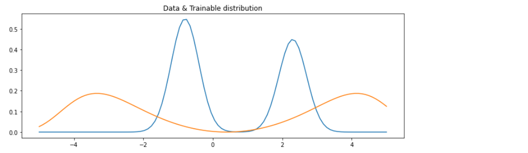
(2) Trainable Distribution 만들기
trainable_dist = tfd.TransformedDistribution(normal,trainable_inv_cubic)
학습시키기 이전의 (초기값의) 분포
x = np.linspace(-5,5,100)
plt.figure(figsize=(12,4))
plt.plot(x,mix_gauss.prob(x),label='data')
plt.plot(x,trainable_dist.prob(x),label='trainable')
plt.title('Data & Trainable distribution')
plt.show()
5-4. Train
-
Optimizer : Adam
-
Loss : **Negative Log likelihood **
num_epochs = 10
opt = tf.keras.optimizers.Adam()
train_losses = []
valid_losses = []

for epoch in range(num_epochs):
    print("Epoch {}...".format(epoch))
    train_loss = tf.keras.metrics.Mean()
    val_loss = tf.keras.metrics.Mean()

    # Train
    for train_batch in x_train:
        with tf.GradientTape() as tape:
            tape.watch(trainable_inv_cubic.trainable_variables)
            loss = -trainable_dist.log_prob(train_batch)
        train_loss(loss)
        grads = tape.gradient(loss, trainable_inv_cubic.trainable_variables)
        opt.apply_gradients(zip(grads, trainable_inv_cubic.trainable_variables))
    train_losses.append(train_loss.result().numpy())

    # Validation
    for valid_batch in x_valid:
        loss = -trainable_dist.log_prob(valid_batch)
        val_loss(loss)
    valid_losses.append(val_loss.result().numpy())
5-5. Result
실제 vs 예측 분포 비교하기
x = np.linspace(-5,5,100)
plt.figure(figsize=(12,4))
plt.plot(x,mix_gauss.prob(x),label='data')
plt.plot(x,trainable_dist.prob(x),label='trainable')
plt.title('Data & Trainable distribution')
plt.show()
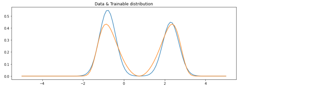
학습된 파라미터는 다음과 같이해서 얻을 수 있다.
trainable_inv_cubic.trainable_variables
(<tf.Variable 'Variable:0' shape=() dtype=float32, numpy=0.5768852>,
 <tf.Variable 'Variable:0' shape=() dtype=float32, numpy=-0.4292613>)