49.Nonparametric Variational Inference (2012)

Nonparametric Variational Inference ( 2012 )

Abstract

Variational Inference : 다루기 쉬운 \(q\)를 사용해서 posterior를 approximate하는 방법

이 논문에서는, “Nonparametric Kernel density estimation” 에서와 같은 방법을 사용하여,

보다 더 complex한 posterior를 근사할 수 있다.

1. Introduction

기존의 VI 방법들과는 달리, 보다 “expressive distribution”을 capture해낼 수 있다.

( 기존의 방법들 ex. Mean Field Variational Inference )

제안한 방법 : NPV (Nonparametric Variational Inference)

• nonparametric한 KDE

• non-conjugate한 상황에서도 사용 가능

• variational family = “Mixture of Gaussian”

  ( Mixture의 다양한 components들은, posterior의 다양한 aspect를 capture할 수 있다 )

• log joint probability의 1차. 2차 미분이 가능해야!

2. Variational Inference

자주 학습했던 내용이니 간단히 언급하고 넘어가겠다.

VI의 objective :

• \(q(\theta)\)와 \(p(\theta \mid y)\)와의 KL-divergence를 minimize하는 것이고,

• 이는 곧 ELBO ( Variational Free Energy)를 maximize하는 것과 같다.

  언제 maximize ? “\(p(\theta \mid y) = q(\theta)\) “

[ ELBO 복습 ]

\(\log p(y)=\mathcal{F}[q]+\mathrm{KL}[q(\theta) \| p(\theta \mid y)]\).

• where \(\mathcal{F}[q]=\mathbb{E}_{q}\left[\log \frac{p(y, \theta)}{q(\theta)}\right]=\mathcal{H}[q]+\mathbb{E}_{q}[f(\theta)]\)
  • \(\mathcal{H}[q]\) : \(q\)의 entropy
  • \(f(\theta)\) = \(\text{log}p(y,\theta)\)

MFVI (Mean Field Variational Inference)

• 자주 사용되는 VI 방법

• \(q(\theta)=\prod_{i} q_{i}\left(\theta_{i}\right)\).

• 장) computational convenience

  단) simple한 posterior approximation & closed form은 conjugate한 경우에만!

3. Nonparametric Variational Inferece

“Flexible family” + “Efficient” inference algorithm

\(q(\theta)\)를 다음과 같은 uniformly weighted Gaussian Mixture로 나타낸다

( isotropic covariance & $N$ : 섞을 Gaussian의 개수 )

\[q(\theta)=\frac{1}{N} \sum_{n=1}^{N} \mathcal{N}\left(\theta ; \mu_{n}, \sigma_{n}^{2} \mathbf{I}\right)\]

이는 마치 nonparametric한 방법의 KDE와 유사하다!

• \(\mu_n\) : kernel center의 역할
• \(\sigma_n^2\) : bandwidth의 역할

3.1 ELBO

ELBO는 closed-form형태로 존재하지 않는 경우가 많다.

\[\mathcal{F}[q]=\mathbb{E}_{q}\left[\log \frac{p(y, \theta)}{q(\theta)}\right]=\mathcal{H}[q]+\mathbb{E}_{q}[f(\theta)]\]

하지만, 우리는 ELBO를 근사할 수 있다! HOW?

• step 1) lower bound \(\mathcal{H}[q]\)( entropy term )
• step 2) approximate \(\mathbb{E}_{q}[f(\theta)]\) ( = \(\mathbb{E}_{q}[\text{log}p(y,\theta)]\) )

위의 step1과 step2를 자세히 들여다보자.

[step 1]

entropy의 lower bound는 Jensen’s inequality를 사용하여, 아래와 같이 구한다.

\(\begin{aligned} \mathcal{H}[q] &=-\int_{\theta} q(\theta) \log q(\theta) d \theta \\ &=-\int_{\theta} q(\theta) \log \frac{1}{N} \sum_{n=1}^{N} \mathcal{N}\left(\theta ; \mu_{n}, \sigma_{n}^{2} \mathbf{I}\right) d \theta \\ & \geq-\frac{1}{N} \sum_{n=1}^{N} \log \int_{\theta} q(\theta) \mathcal{N}\left(\theta ; \mu_{n}, \sigma_{n}^{2} \mathbf{I}\right) d \theta \end{aligned}\).

$\therefore$ \(\mathcal{H}[q] \geq-\frac{1}{N} \sum_{n=1}^{N} \log q_{n}\).

• where \(q_{n}=\frac{1}{N} \sum_{j=1}^{N} \mathcal{N}\left(\mu_{n} ; \mu_{j},\left(\sigma_{n}^{2}+\sigma_{j}^{2}\right) \mathbf{I}\right)\)

[step 2]

ELBO의 두번째 term인 expected log joint \(f(\theta)\)를 살펴보자.

\(\mathbb{E}_{q}[f(\theta)]=\frac{1}{N} \sum_{n=1}^{N} \int_{\theta} \mathcal{N}\left(\theta ; \mu_{n}, \sigma_{n}^{2} \mathbf{I}\right) f(\theta) d \theta\).

Taylor series expansion을 사용하여, 아래와 같이 근사할 수 있다.

\(\begin{aligned} f(\theta) \approx \hat{f}_{n}(\theta)=& f\left(\mu_{n}\right)+\nabla f\left(\mu_{n}\right)\left(\theta-\mu_{n}\right)+ \frac{1}{2}\left(\theta-\mu_{n}\right)^{\top} \mathbf{H}_{n}\left(\theta-\mu_{n}\right) \end{aligned}\).

\(\begin{aligned}\mathbb{E}_{q}[f(\theta)] &\approx \mathbb{E}_{q}[\hat{f}(\theta)] &\\&=\frac{1}{N} \sum_{n=1}^{N} \int_{\theta} \mathcal{N}\left(\theta ; \mu_{n}, \sigma_{n}^{2} \mathbf{I}\right) \hat{f}_{n}(\theta) d \theta \\&=\frac{1}{N} \sum_{n=1}^{N} f\left(\mu_{n}\right)+\frac{\sigma_{n}^{2}}{2} \operatorname{Tr}\left(\mathbf{H}_{n}\right)\end{aligned}\).

(요약) 위의 Step1과 Step2를 통해, 우리는 ELBO를 아래와 같이 근사할 수 있다.

• 1차 근사 : \(\mathcal{L}_{1}[q]=\frac{1}{N} \sum_{n=1}^{N} (f\left(\mu_{n}\right)-\log q_{n})\)

• 2차 근사 : \(\mathcal{L}_{2}[q]=\frac{1}{N} \sum_{n=1}^{N} (f\left(\mu_{n}\right)+\frac{\sigma_{n}^{2}}{2} \operatorname{Tr}\left(\mathbf{H}_{n}\right)-\log q_{n})\).

  • (1) likelihood term
  • (2) Hessian term
  • (3) entropy term

  으로 분해할 수 있는 것을 확인할 수 있다 :)

ELBO를 근사하는 2가지 장점?

• 1) conjugacy assumption이 필요 없다

  ( 단지 \(f(\theta) = \text{log}p(\theta,y)\)가 2번 미분가능하기만 하면 된다 )

• 2) Hessian term을 가지고 있긴 하지만, 오직 대각 요소만을 계산하면 된다

  ( gradient를 계산하는 것 보다 더 적은 computation 소요 )

3.2 Optimizing ELBO

앞서서 근사한 ELBO를, variational parameter인 \(\mu_n\)과 \(\sigma_n\)에 대해서 최적화하면 된다.

gradient-based방법을 사용해도 되지만, 이는 computational problem이 있기 때문에 ( Hessian의 trace의 gradient를 계산하기 위해 3번 미분해야 하므로 )

우리는 아래와 같은 방법으로 최적화한다 (1차,2차 근사만 사용!)

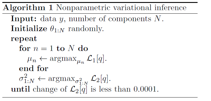
이처럼, 최적화 문제를 2단계로 나눠서 품에 따라, (3차 근사까지하지 않고도) 연산량을 절감할 수 있다

NPV에 필요한 parameter수는, \(N\)에 따라 linear하게 증가한다.

( hidden variable이 많은 model에는 어려울 수 있음 )

posterior의 major aspect를 capture해내고 싶다면, 적은 수의 component만을 사용할 필요가 있다.

3.3 Relationship to other algorithms

\(N=1\)이고 \(\sigma_1 \rightarrow 0\)

• \(\mathcal{L}[q]=\log p(y, \mu)+\text { const. }=\log p(\theta=\mu \mid y)+\text { const}\).
• 이는 곧 “MAP” solution
• diagonalized Laplace approximation으로 볼 수도 있다

\(N>1\)이고 \(\sigma_n \rightarrow 0\)

• \(q(\theta)=\frac{1}{N} \sum_{n=1}^{N} \delta_{\mu_{n}}(\theta)\).

  ( \(\delta_{\mu_{n}}(\cdot)\) : Dirac point mass located at \(\mu_{n}\) )

• posterior에 대한 quasi-Monte Carlo approximation과 동일하다

• deterministic한 sampling 방법으로 볼 수도 있다.