Variational Inference in Nonconjugate Models ( 2013 )

Abstract

MFVI는 자주 사용되는 VI 방법으로서, coordinate-ascent algorithm을 사용한다. 하지만 이것은 conditionally conjugate한 경우에만 closed-form 형태로 존재한다. 그러나 대부분의 모델은 non-conjugate하다.

따라서, 이 논문에는 *non-conjugate model을 위한 2가지 generic method를 제안한다.

1) Laplace Variational Inference
2) Delta method Variational Inference

위 두 방법에 대해 설명한 뒤, 이를 세 가지 모델에 적용해서 설명할 것이다.

1) Correlated Topic model
2) Bayesian Logistic Regression
3) Hierarchical Bayesian Logistic Regression

1. Introduction

대부분의 경우는 non-conjugate하다. 따라서 VI를 이에 적용하고자 한다면, 특정 모델에 맞춤형으로 알고리즘을 설계해야 한다. 따라서 이 논문은, MFVI에 2가지 방법을 사용하여(Laplace VI, delta method VI) 많은 non-conjugate 모델에 적용가능하도록 알고리즘을 설계한다.

그런 뒤, 앞서 말한 3가지 non-conjugate 모델에 이를 적용해 볼 것이다

(Correlated Topic model, Bayesian Logistic Regression, Hierarchical Bayesian Logistic Regression)

2. Variational Inference and a Class of Nonconjugate Models

notation

$x$ : observation
$\theta,z$ : hidden variable

$\rightarrow$ $p(\theta, z, x)=p(x \mid z) p(z \mid \theta) p(\theta)$

이 단원에서는 다음의 2가지에 대해 설명 (복습)할 것이다.

2-1. MFVI

가장 자주 사용되는 간단한 VI 방법으로, MFVI (Mean Field Variational Inference)가 있다.

이는 (1) fully factorized variational family를 설정하고, (2) 각각의 latent variable은 서로 independent함을 가정한다.

우리의 목표는 KL divergence를 최소화하는 것으로, ELBO를 최대화 하는 것과 동일하다.

ELBO는 Jensen’s inequality를 통해 알 수 있다.

$\begin{aligned} \log p(x) &=\log \int p(\theta, z, x) \mathrm{d} z \mathrm{~d} \theta \\ & \geq \mathbb{E}_{q}[\log p(\theta, z, x)]-\mathbb{E}_{q}[\log q(\theta, z)] \\ & \triangleq \mathcal{L}(q) \end{aligned}$.

이를 풀면, 우리는 다음의 optimal solution을 찾을 수 있따.

$\begin{array}{l} q^{*}(\theta) \propto \exp \left\{\mathbb{E}_{q(z)}[\log p(z \mid \theta) p(\theta)]\right\} \\ q^{*}(z) \propto \exp \left\{\mathbb{E}_{q(\theta)}[\log p(x \mid z) p(z \mid \theta)]\right\} . \end{array}$.

그런 뒤, coordinate ascent algorithm을 통해 iterative하게 $\theta$와 $z$를 update한다.

( $q(z)$를 update하는 동안 $\theta$를 fix, vise versa )

이러한 coordinate update는, 모델이 conditionally conjugate한 경우에만 closed-form형태로 풀 수 있다. 하지만, 대부분의 모델은 그러하지 않기 때문에 , 이 논문은 wide class of non-conjugate 모델에 적용 가능한 generic variational inference 알고리즘을 제안한다.

2-2. A class of Non-conjugate Models

우리는 $p(\theta, z, x)=p(x \mid z) p(z \mid \theta) p(\theta)$를 그대로 가정한 채로, 아래의 가정을 만족하는 다양한 non-conjugate 모델을 대상으로 할 것이다.

가정 1) $p(\theta)$ 는 $\theta$에 대해 2차 미분가능하다
가정 2) $p(z\mid \theta)$는 exponential family이다
가정 2) $p(x\mid z)$는 exponential family이다

여기서

$\theta$는 non-conjugate variable
$z$는 conjugate variable
$x$는 observation 이다

이러한 모델에 해당하는 예로는, “correlated topic model”, “dynamic topic model”, “Bayesian Logistic Regression”,”Discrete Choice models” 등이 있다.

ex) Hierarchical Language model

간단한 non-conjugate한 모델의 예시이다
unigram language modeling을 푸는 모델이다
- prior : Dirichlet

다음과 같은 step으로 작동한다

step 1) draw log Dirichlet Parameters, $\theta \sim \mathcal{N}(0, I)$
step 2) for each document $d$, $1 \leq d \leq D$
step 3) draw multinomial parameter , $z_{d} \mid \theta \sim$ Dirichlet $(\exp \{\theta\})$.
step 4) draw word counts, $x_{d} \sim$ Multinomial $\left(N, z_{d}\right)$.

문서들의 collection이 주어졌을 때, posterior $p\left(\theta, z_{1: D} \mid x_{1: D}\right)$를 계산하는 것이 목적이다.

3.Laplace and Delta method Variational Inference

Laplace & Delta method 위 두가지 방법 모두 coordinate ascent방법을 사용하여 optimize한다 ( 즉, iterative update between $q(\theta)$ and $q(z)$ )

또한, 이 둘 다 variational distribution이 mean-field family임을 가정한다.
이 둘의 차이는, $q(\theta)$를 update하는 방식에 있다.

Laplace : $\begin{array}{l} q^{*}(\theta) \propto \exp \left\{\mathbb{E}_{q(z)}[\log p(z \mid \theta) p(\theta)]\right\} \\ q^{*}(z) \propto \exp \left\{\mathbb{E}_{q(\theta)}[\log p(x \mid z) p(z \mid \theta)]\right\} . \end{array}$. 에 Laplace approximation 적용
Delta method : $\begin{aligned} \log p(x) &=\log \int p(\theta, z, x) \mathrm{d} z \mathrm{~d} \theta \\ & \geq \mathbb{E}_{q}[\log p(\theta, z, x)]-\mathbb{E}_{q}[\log q(\theta, z)] \\ & \triangleq \mathcal{L}(q) \end{aligned}$ 에 Taylor expansion 적용

이 두 가지 방법에서 모두 complete variational family는 아래와 같다.

$q(\theta, z)=q(\theta \mid \mu, \Sigma) q(z \mid \phi)$.

3-1. Laplace Variational Inference

3-1-1. Laplace Approximation

intractable density를 Gaussian을 사용해서 근사한다.

그러기 위해, MAP point에서 Taylor approximation을 적용한다.

우선, posterior는 exponential log joint에 proportional 하다.

$p(\theta \mid x)=\exp \{\log p(\theta \mid x)\} \propto \exp \{\log p(\theta, x)\}$.

$\hat{\theta}$를 $p(\theta \mid x)$의 MAP라고 하면, Taylor series expansion을 아래와 같이 나타낼 수 있다.

$\log p(\theta \mid x) \approx \log p(\hat{\theta} \mid x)+\frac{1}{2}(\theta-\hat{\theta})^{\top} H(\hat{\theta})(\theta-\hat{\theta})$.

$H(\hat{\theta})$는 $\hat{\theta}$에서 측정한 $\log p(\theta \mid x)$의 Hessian이다.
MAP이기 때문에, 1차 미분한 값 ($\nabla \log p(\theta \mid x)\mid_{\theta=\hat{\theta}}$)는 0이 된다.

따라서 $$\left.(\theta-\hat{\theta})^{\top} \nabla \log p(\theta \mid x)\right _{\theta=\hat{\theta}}$$도 0이다.

위 식을 통해 Gaussian에 근사할 수 있다.

$p(\theta \mid x) \approx \frac{1}{C} \exp \left\{-\frac{1}{2}(\theta-\hat{\theta})^{\top}(-H(\hat{\theta}))(\theta-\hat{\theta})\right\}$.

$\therefore$ $p(\theta \mid x) \approx \mathcal{N}\left(\hat{\theta},-H(\hat{\theta})^{-1}\right)$.

3-1-2. Laplace Updates in Variational Inference

$p(z \mid \theta)=h(z) \exp \left\{\eta(\theta)^{\top} t(z)-a(\eta(\theta))\right\}$ … exponential family 형태
$q^{*}(\theta) \propto \exp \left\{\mathbb{E}_{q(z)}[\log p(z \mid \theta) p(\theta)]\right\}$ ….. exp(log joint)에 proportional

이 두 식을 결합하면, 우리는 아래와 같이 나타낼 수 있다.

$q(\theta) \propto \exp \left\{\eta(\theta)^{\top} \mathbb{E}_{q(z)}[t(z)]-a(\eta(\theta))+\log p(\theta)\right\}$.

let $f(\theta) \triangleq \eta(\theta)^{\top} \mathbb{E}_{q(z)}[t(z)]-a(\eta(\theta))+\log p(\theta)$
$q(\theta) \propto \exp \{f(\theta)\}$.

$\rightarrow$ 이 식은 closed form으로 풀리지 않기 때문에, Taylor approximation을 통해 2차 근사한다.

$f(\theta) \approx f(\hat{\theta})+\nabla f(\hat{\theta})(\theta-\hat{\theta})+\frac{1}{2}(\theta-\hat{\theta})^{\top} \nabla^{2} f(\hat{\theta})(\theta-\hat{\theta})$.

$q(\theta) \propto \exp \{f(\theta)\} \approx \exp \left\{f(\hat{\theta})+\frac{1}{2}(\theta-\hat{\theta})^{\top} \nabla^{2} f(\hat{\theta})(\theta-\hat{\theta})\right\}$.

$\therefore$ $q(\theta) \approx \mathcal{N}\left(\hat{\theta},-\nabla^{2} f(\hat{\theta})^{-1}\right)$.

위 식을 통해, 우리는 non-conjugate한 모델에도 coordinate ascent algorithm을 적용할 수 있다.

3-2. Delta Method Variational Inference

Delta method는 Laplace method와 다르게, ”$L$ (ELBO)”에 Taylor series expansion을 적용한다.

$p(z \mid \theta)=h(z) \exp \left\{\eta(\theta)^{\top} t(z)-a(\eta(\theta))\right\}$.
$\mathcal{L}(q) = \mathbb{E}_{q}[\log p(\theta, z, x)]-\mathbb{E}_{q}[\log q(\theta, z)]$.

이 두 식을 사용하여, 우리는 아래와 같이 나타낼 수 있다.

$\mathcal{L}(q(\theta))=\mathbb{E}_{q(\theta)}\left[\eta(\theta)^{\top} \mathbb{E}_{q(z)}[t(z)]-a(\eta(\theta))+\log p(\theta)\right]+\frac{1}{2} \log \mid \Sigma \mid$.

1번째 term : $\mathbb{E}_{q(\theta)}[f(\theta)]$
2번째 term : Gaussian의 entropy에서 나온다. ( $-\mathbb{E}_{q(\theta)}[\log q(\theta)]=\frac{1}{2} \log \mid \Sigma \mid+C$ )

이를 다시 적은 뒤, Taylor Approximation을 통해 다음과 같이 근사할 수 있다.

$\mathcal{L}(q(\theta))=\mathbb{E}_{q(\theta)}[f(\theta)]+\frac{1}{2} \log \mid \Sigma \mid$.

$\left.\left.\mathcal{L}(q(\theta)) \approx f(\hat{\theta})+\nabla f(\hat{\theta})^{\top}(\mu-\hat{\theta})+\frac{1}{2}(\mu-\hat{\theta})^{\top} \nabla^{2} f(\hat{\theta})(\mu-\hat{\theta})\right]\right]+\frac{1}{2}\left(\operatorname{Tr}\left\{\nabla^{2} f(\hat{\theta}) \Sigma\right\}+\log \mid \Sigma \mid \right)$.

여기서 우리는 $\hat{\theta}$를 선택해야 한다.

후보 1) $\hat{\theta}=$ maximum of $f(\theta)$
후보 2) $\hat{\theta}=$ mean of the distribution from previous iteration of coordinate ascent
후보 3) $\hat{\theta}=\mu$ ( = mean of the variational distribution $q(\theta)$ )

이 중 후보3) $\hat{\theta}=\mu$를 사용한다. 그러면 우리의 objective (ELBO)는 아래와 같이 나타내진다.

$\mathcal{L}(q(\theta)) \approx f(\mu)+\frac{1}{2} \operatorname{Tr}\left\{\nabla^{2} f(\mu) \Sigma\right\}+\frac{1}{2} \log \mid \Sigma \mid$.

3-3. Updating the Conjugate Variable

지금까지 non-conjugate variable $q(\theta)$에 대한 variational update를 하는 2가지 방법에 대해 살펴봤다. 이제는 conjugate variable $q(z)$에 대해서 update를 할 것이다.
아래의 두 식을 사용하여, $\text{log}q(z)$ 를 정리하면 다음과 같다.

$q^{*}(z) \propto \exp \left\{\mathbb{E}_{q(\theta)}[\log p(x \mid z) p(z \mid \theta)]\right\}$.
$p(z \mid \theta)=h(z) \exp \left\{\eta(\theta)^{\top} t(z)-a(\eta(\theta))\right\}$.

$\rightarrow$ $\log q(z)=\log p(x \mid z)+\log h(z)+\mathbb{E}_{q(\theta)}[\eta(\theta)]^{\top} t(z)+C$.

따라서, $q(z) \propto h(z) \exp \left\{\left(\mathbb{E}_{q(\theta)}[\eta(\theta)]+t(x)\right)^{\top} t(z)\right\}$가 된다.

이것이 $q(z)$에 대한 update이다.

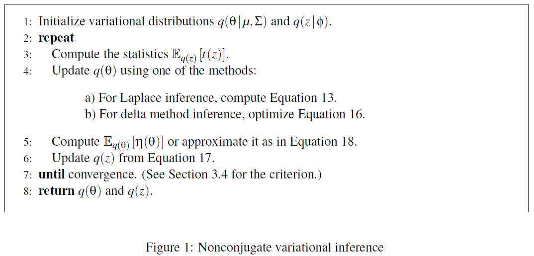
3-4. Nonconjugate Variational Inference

Nonconjugate Variational inference의 full-algorithm에 대해 소개하겠다.

nonconjugate variable은 Gaussian $q(\theta \mid \mu, \Sigma)$
conjugate variable은 $q(z \mid \theta)$이다.

알고리즘은 아래와 같다.

4. Example Models

지금까지 배운 것을 다음의 3가지 모델에 적용해 볼 것이다.

4-1. Correlated Topic Model

Probabilistic topic models

models of document collection
each document = group of observed words ( that are drawn from mixture model )
topics = mixture components : distribution over terms that are shared for the whole collection

그 중에서, CTM (Correlated Topic Model)에 대해 설명을 하겠다.

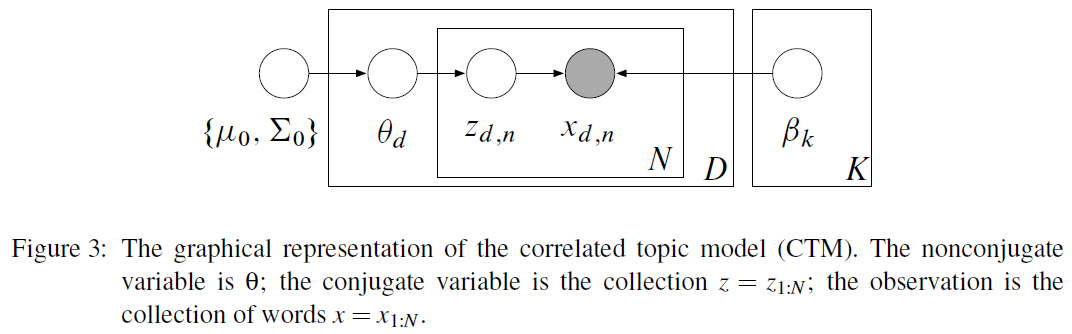
이 모델은 아래와 같은 순서로 진행된다.

1) draw log topic proportion : $\theta \sim \mathbf{N}(\mu_0, \Sigma_0)$
2) for each word $n$:
- 1) draw topic assignment : $z_n \mid \theta \sim \text{Mult}(\pi(\theta))$
- 2) draw word $x_n \mid z_n, \beta \sim \text{Mult}(\beta_{z_n})$

(topic proportion) $\theta$에 대한 분포는 Gaussian이다 : $q(\theta) = \mathbf{\mu,\Sigma}$

(topic assignment) $z$에 대한 분포는 discrete 하다 : $q(z) = \prod_n q(z_n \mid \phi_n)$

4-2. Bayesian Logistic Regression

binary classification을 위한 모델로써, Gaussian prior를 사용한다

아래와 같은 순서로 진행된다

1) draw coefficients $\theta \sim \mathcal{N}\left(\mu_{0}, \Sigma_{0}\right)$
2) for each data point $n$ & covariates $t_n$ , draw its class label from

$z_{n} \mid \theta, t_{n} \sim \operatorname{Bernoulli}\left(\sigma\left(\theta^{\top} t_{n}\right)^{z_{n, 1}} \sigma\left(-\theta^{\top} t_{n}\right)^{z_{n, 2}}\right)$.

where $\sigma(y) \triangleq 1 /(1+\exp (-y))$ ( = logistic function)

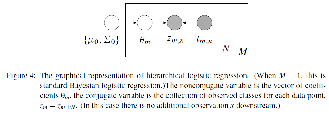
4-3. Hierarchical Bayesian Logistic Regression

위의 4-2를 확장한 것이다.