54.Doubly Stochastic Variational Bayes for non-Conjugate Inference (2014)

Doubly Stochastic Variational Bayes for non-Conjugate Inference ( 2014 )

Abstract

이 논문은, Bayesian non-conjugate inference에 적용 가능한, stochastic optimization에 기반한 “Simple & Effective” variational inference방법을 제안한다. 여기서 제안한 알고리즘을 아래의 2가지 예시에 적용하여 설명한다.

• 1) Variable selection in logistic regression
• 2) Fully Bayesian inference over kernel hyperparameters in Gaussian process regression

1. Introduction

많은 ML문제들은 “complex”한 모델을 “large scale”에 적용하고 싶어한다.

이때, Bayesian computation방법은 (conjugate한 모델을 제외하고는) intractable하기 때문에, 아래와 같이 크게 2가지 방법으로 approximation(근사)해서 문제를 대신 푼다.

• 1) MCMC

  • unbiased estimate를 제공한다
  • slow

• 2) Variational Bayesian Inference

  • optimization문제로 치환해서 푼다

  • fast

  • ELBO는 high dimensional expectation을 요구!

    ( 이는 intractable for non-conjugate model )

이 논문은 Variational Inference의 적용 범위를 확장시킨다. HOW?

“By introducing a simple stochastic optimization algorithm, that can be widely applied in non-conjugate models, where the joint probability densities are differentiable functions of the parameters “

기존의 non-conjugate stochastic variational inference와의 차이점은, “model joint density”의 gradient를 사용한다는 점이다.

stochasticity를 부여하는 방법에 있어서도 기존의 방법과 차이가 있는데, 기존에는 data sub-sampling을 통해 stochasticity를 부여했다면, 이 방법은 variational distribution으로부터의 sampling을 통해 stochasticity를 부여한다.

이 두 가지의 stochasticity를 combine하여,어떻게 “doubly stochastic variational inference” 알고리즘을 만드는지, 그리고 더 나아가서 이것이 어떻게 large scale problem에서 non-conjugate inference를 하는지에 대해 설명할 것이다.

2. Theory

[1] 첫 째, \(\phi(\mathbf{z})\)분포를 따르는 random vector \(\mathbf{z}\)가 있다고 가정해보자. 이것의 mean vector는 0이고, scale parameter는 0이라고 하자.

이떄, 우리는 \(\phi(\mathbf{z})\)를 standard distribution이라고 한다.

[2] 둘 째, \(\phi(\mathbf{z})\)에서 independent한 sample이 뽑는 것이 가능하다고 하자.

우리는 이 \(\phi(\mathbf{z})\)를 building block으로 하여, variational distribution을 만들어 나갈 것이다.

현재 \(\phi(\mathbf{z})\)는 standard distribution으로써 특별한 structure가 없지만, 아래와 같은 invertible transformation을 통해 structure를 만들어 나갈 수 있다.

\(\theta=C \mathbf{z}+\mu\). ( 혹은, \(\mathbf{z} = C^{-1}(\theta-\mu)\) )

• 여기서 \(C\)는, lower triangular positive definite matrix이다.
  

[3] Variable Transformation에 의해, \(\theta\)에 대한 distribution은 Jacobian을 곱해서 아래와 같이 나타낼 수 있다.

\(q(\theta \mid \mu, C)=\frac{1}{\mid C \mid} \phi\left(C^{-1}(\theta-\mu)\right)\).

• 이 분포는 parameter로써 mean vector \(\mu\)와 scale matrix \(C\)를 가지고 있다.
• 이 분포 (\(q(\theta \mid \mu, C)\))를 우리의 variational distribution을 근사하는 데에 사용할 것이다.
  

[4] 마지막으로, 아래와 같은 joint density를 가진 probabilistic model을 가정할 것이다.

\(g(\boldsymbol{\theta})=p(\mathbf{y} \mid \boldsymbol{\theta}) p(\boldsymbol{\theta})=p(\mathbf{y}, \boldsymbol{\theta})\).

• \(\mathbf{y}\) : data

• \(\theta\) : \(D\)차원의 unobserved random variable

  ( latent variable과 parameter를 모두 포함한다 )
  

우리의 목표는 KL-divergence \(\operatorname{KL}[q(\theta \mid \mu, C) \| p(\theta \mid \mathrm{y})]\)를 최소화하는 것이다.

이는, 다음의 ELBO를 maximize하는 것과 동일하다.

\(\mathcal{F}(\boldsymbol{\mu}, C)=\int q(\boldsymbol{\theta} \mid \boldsymbol{\mu}, C) \log \frac{g(\boldsymbol{\theta})}{q(\boldsymbol{\theta} \mid \boldsymbol{\mu}, C)} d \boldsymbol{\theta}\).

이 ELBO에, variable transformation ( \(\theta=C \mathbf{z}+\mu\). ( 혹은, \(\mathbf{z} = C^{-1}(\theta-\mu)\) ) )을 적용하면,

\(\begin{aligned} \mathcal{F}(\boldsymbol{\mu}, C) &=\int \boldsymbol{\phi}(\mathbf{z}) \log \frac{g(C \mathbf{z}+\boldsymbol{\mu})|C|}{\phi(\mathbf{z})} d \mathbf{z} \\ &=\mathbb{E}_{\boldsymbol{\phi}(\mathbf{z})}[\log g(C \mathbf{z}+\boldsymbol{\mu})]+\log |C|+\mathcal{H}_{\phi} \end{aligned}\).

• $$\log

  C

  =\sum_{d=1}^{D} \log C_{d d}$$.

• \(\mathcal{H}_{\phi}\) : entropy of \(\phi(z)\).

위 ELBO 식 ( \(\mathcal{F}(\boldsymbol{\mu}, C) =\mathbb{E}_{\boldsymbol{\phi}(\mathbf{z})}[\log g(C \mathbf{z}+\boldsymbol{\mu})]+\log \mid C\mid+\mathcal{H}_{\phi}\) )를 \(\mu\)와 \(C\)에 대해서 미분하면, 아래와 같다.

• \(\nabla_{\mu} \mathcal{F}(\mu, C)=\mathbb{E}_{\phi(\mathbf{z})}\left[\nabla_{\mu} \log g(C \mathbf{z}+\mu)\right]\).
• \(\nabla_{C} \mathcal{F}(\mu, C)=\mathbb{E}_{\phi(\mathbf{z})}\left[\nabla_{C} \log g(C \mathbf{z}+\mu)\right]+\Delta_{C}\).
  • \(\Delta_{C}\) : diagonal matrix with elements \(\left(1 / C_{11}, \ldots, 1 / C_{D D}\right)\) in diagonal
    

우리는 chain rule을 통해, 아래와 같이\(C\mathbf{z} + \mu\)가 들어가게끔 재표현할 수 있다.

• \(\nabla_{\mu} \log g(C \mathbf{z}+\mu)=\nabla_{C \mathbf{z}+\mu} \log g(C \mathbf{z}+\mu)\).
• \(\nabla_{C}^{} \log g(C \mathbf{z}+\mu)=\nabla_{C \mathbf{z}+\mu} \log g(C \mathbf{z}+\mu) \mathbf{z}^{T}\).
  

이를 위의 \(\nabla_{\mu} \mathcal{F}(\mu, C)\)와 \(\nabla_{C} \mathcal{F}(\mu, C)\)에 대입하면, 아래와 같이 \(\theta\)에 대해서 나타낼 수 있다.

• \(\nabla_{\boldsymbol{\mu}} \mathcal{F}(\boldsymbol{\mu}, C) =\mathbb{E}_{q(\boldsymbol{\theta} \mid \boldsymbol{\mu}, C)}\left[\nabla_{\boldsymbol{\theta}} \log g(\boldsymbol{\theta})\right]\).

• \(\nabla_{C} \mathcal{F}(\boldsymbol{\mu}, C) =\mathbb{E}_{q(\boldsymbol{\theta} \mid \boldsymbol{\mu}, C)}\left[\nabla_{\boldsymbol{\theta}} \log g(\boldsymbol{\theta}) \times(\boldsymbol{\theta}-\boldsymbol{\mu})^{T} C^{-T}\right] +\Delta_{C}\).

지금까지 설명한 것을 바탕으로, DSVI (Doubly Stochastic Variational Inference) 알고리즘의 단계를 요약하면, 아래와 같다.

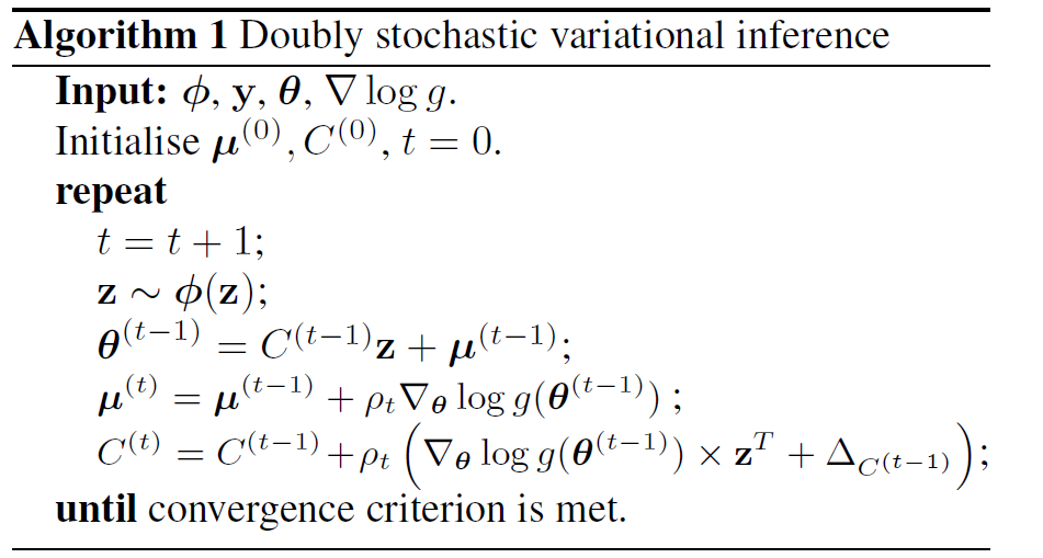
위 알고리즘이 “Doubly Stochastic”인 이유는, 기존의 stochastic variational inference와는 다르게, 2가지 방향에서 stochasticity가 나타나기 때문이다.

• 기존) training data의 sub-sampling을 통해 생성된 mini batch를 통한 online parameter update
• DSVI ) sampling “from the variational distribution”

( joint probability model의 경우, 이 두가지의 stochasticity 를 모두 사용할 수 있다 )

\(\theta\)의 차원이 매우 큰 경에는, full scale matrix \(C\)를 사용하는 것은 impractical 하기 때문에, 이것 대신 diagonal matrix를 사용할 수 있다. 그럴 경우, 위 알고리즘 식에서 \(C\)의 updating equation은 다음과 같이 변경되면 된다.

\(c_{d}^{(t)}=c_{d}^{(t-1)}+\rho_{t}\left(\frac{\partial \log g\left(\boldsymbol{\theta}^{(t-1)}\right)}{\partial \theta_{d}} z_{d}+\frac{1}{c_{d}^{(t-1)}}\right)\).

​ where \(d=1, \ldots, D\)

2-1. Connection with the Gaussian approximation

Variational distribution으로서 Gaussian을 설정할 경우 ( = \(\mathcal{N}(\theta \mid \mu, \Sigma)\) )의 Lower Bound는 아래와 같다.

\(\mathcal{F}(\boldsymbol{\mu}, \Sigma)=\int \mathcal{N}(\boldsymbol{\theta} \mid \boldsymbol{\mu}, \Sigma) \log \frac{g(\boldsymbol{\theta})}{\mathcal{N}(\boldsymbol{\theta} \mid \boldsymbol{\mu}, \Sigma)} d \boldsymbol{\theta}\).

아래의 두 조건을 충족시킬 경우,

• paramterization \(\Sigma = CC^T\)
• \(\text{log}g(\theta)\) 는 concave function

\(\rightarrow\) bound is concave w.r.t \((\mu,C)!\)

( 하지만, 이 제약으로 인해 보다 복잡한 모델링이 제한된다. )

이에 반해, 이 논문에서 제안한 stochastic variational framework는, \(\text{log}g(\theta)\)가 단지 \(\theta\)에 대해 미분가능할 것만을 요구한다.

\(\phi(\mathbf{z})\)가 standard normal \(\mathbf{N}(\mathbf{z} \mid 0,I)\) 를 따를 경우, ELBO인 \(\mathcal{F}(\boldsymbol{\mu}, C) =\mathbb{E}_{\boldsymbol{\phi}(\mathbf{z})}[\log g(C \mathbf{z}+\boldsymbol{\mu})]+\log \mid C \mid+\mathcal{H}_{\phi}\)는 Gaussian Approximation이 된다!

그런 뒤, 위의 DSVI iteration을 적용하면 이는 Gaussian Approximation bound를 최대화 할 수 있다.

따라서, DSVI는 Gaussian Approximation을 보다 많은 모델에 적용할 수 있게끔 한다.

뒤에 내용 Skip