Smoothed Gradients for Stochastic Variational Inference ( 2014 )
Abstract
SVI (Stochastic Variational Inference) 는 scalable한 Bayesian Computation방법이다. 이 방법은 stochastic optimization을 통해 noisy natural gradient을 쉽게 계산할 수 있다. 여기서, 우리는 SVI가 “unbiased” stochastic gradient를 갖도록 신경써야했다.
하지만 이 논문은, BIASED된 stochastic gradient를 사용하는 SVI를 제안한다. 결론부터 말하자면,bias를 용인하는 대신 variance를 (그 이상으로) reduce하는 효과를 가져온다. 기존의 natural gradient를, 이전 몇개의 term들의 fixed-window moving average를 통해 이와 비슷한 gradient로 대체한다.
이 방법의 장점은 아래와 같다.
-
1) computational cost는 기존의 SVI와 동일하다
( + storage requirement도 상수배 만큼만 더 요구될 뿐이다 )
-
2)
- 기존의 unbiased gradient보다는 “Variance Reduction”효과를,
- 기존의 averaged gradient보다는 “Smaller Bias”를
- 기존의 full gradient보다는 “Smaller MSE”를 가진다!
여기서 제안한 알고리즘을 LDA를 사용해 test한다.
1. Introduction
( SVI에 대한 소개는 Abstract로 충분하므로 생략한다 )
이 논문은 BIASED된 stochastic gradient를 사용한다. 하지만, 이전에도 biased된 gradient를 사용한 알고리즘들이 있었다. (ex : SAG, AG) 하지만, SAG와 AG 모두 SVI에 아주 applicable하지는 않았다.
1) SAG :모든 gradient를 store할 것을 요구했다
2) AG : SVI update는 기존의 파라미터와 새로운 noisy version간의 convex combination으로 update가 되었지만, AG는 이 요건을 충족하지 못한다.
이 논문에서 제시한 Smoothed Gradients에 대해 이해하기 전에, variational parameter \(\lambda_i\)가 update되는 과정을 한번 잘 살펴보자.
notation
-
\(\lambda_i\) : 현재 시점 (\(i\))에서의 variational parameter
-
\(w_i\) : data point
-
\(\hat{S_i}\) : \(\lambda_i\)를 통해 측정된 \(w_i\)에 대한 sufficient statistic
( \(\lambda_i\)와 같은 dimension을 가진다 )
- \(\eta\) : prior from the model
- \(N\) : appropriate scaling
우리의 Variational objective \(\mathcal{L}\)은 아래와 같이 simple하다!
\(\nabla_{\lambda} \mathcal{L}=\eta+ N \hat{S}_{i}-\lambda_{i}\).
위 식은, UNBIASED된 noisy gradient이다. 이를 ( iteration에 따라 점차 감소하는 ) step size \(\rho_i\)에 따라 updating equation을 세운다면, 아래와 같다.
\(\lambda_{i+1}=\left(1-\rho_{i}\right) \lambda_{i}+\rho_{i}\left(\eta+N \hat{S}_{i}\right)\).
방금 설명한 위 식의 구조를 잘 이해하길 바란다.
여기서 제안한 알고리즘은, 위 식에서의 natural gradient를, 앞선 \(L\)개의 sufficient statistic의 fixed-window moving average로 대체한다.
( 즉, \(N \hat{S}_{i}\) 대신 \(\mathrm{m}, \sum_{j=0}^{L-1} \hat{S}_{i-j}\)를 사용한다 )
이럴 경우의 장점은, 위의 Abstarct에서 설명했다. 이제 이 알고리즘에 대한 세부적인 내용에 대해서 이야기하겠다.
2. Smoothed stochastic gradients for SVI
LDA & VI
LDA에 대해 빠르게 짚고 넘어가겠다. 우선, notation을 아래와 같이 정의한다.
- \(D\) documents with words \(w_{1:D,1:N}\)
- \(K\) hidden topics ( followed by Multinomial Distn )
- \(V\) vocabulary size
- multinomial parameter \(\beta_{1:V,1:K}\)
각각의 document \(d\)는, topic weights \(\Theta_d\) 를 가지고 있다.
document \(d\)에 속한 word \(n\)은 topic assignment \(z_{dn}\)을 가지고 있다 ( K-vector of binary entries )
( \(z_{dn}^k=1\) if word \(n\) in documnet \(d\) is assigned to topic \(k\), \(z_{dn}^k=0\) otherwise )
다음과 같은 step으로 진행된다.
-
(1) draw topics : \(\beta_{k} \sim\) Dirichlet \((\eta)\)
-
(2) draw topic weights, for each document : \(\Theta_{d} \sim\) Dirichlet \((\alpha)\)
-
(3) draw an assignment , for each word in each document : \(z_{d n} \sim\) Multinomial \(\left(\Theta_{d}\right)\)
-
(4) draw a word from the assigned topic : \(w_{d n} \sim\) Multinomial \(\left(\beta_{z_{d n}}\right)\)
Joint pdf는, 아래와 같이 factorize될 수 있다.
\(p(w, \beta, \Theta, z \mid \eta, \alpha)=\prod_{k=1}^{K} p\left(\beta_{k} \mid \eta\right) \prod_{d=1}^{D} p\left(\Theta_{d} \mid \alpha\right) \prod_{n=1}^{N} p\left(z_{d n} \mid \Theta_{d}\right) p\left(w_{d n} \mid \beta_{1: K}, z_{d n}\right)\).
이를 쉽게 graphical model representation으로나타내면 아래와 같다.
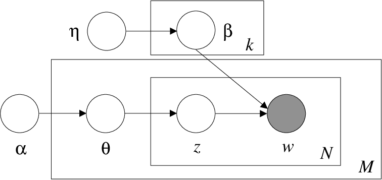
위 모델의 posterior는 아래와 같이 나타낼 수 있다
\(p(\beta, \Theta, z \mid w)=\frac{p(\beta, \Theta, z, w)}{\sum_{z} \int d \beta d \Theta p(\beta, \Theta, z, w)}\).
하지만 위 식은 intractable하기 때문에, 우리는 아래의 factorzied distribution \(q\)로 근사해서 푼다.
\(q(\beta, \Theta, z)=q(\beta \mid \lambda)\left(\prod_{d=1}^{D} \prod_{n=1}^{N} q\left(z_{d n} \mid \phi_{d n}\right)\right)\left(\prod_{d=1}^{D} q\left(\Theta_{d} \mid \gamma_{d}\right)\right)\).
- \(q(\beta \mid \lambda)\)와 \(q\left(\Theta_{d} \mid \gamma_{d}\right)\)는 Dirichlet distribution
- \(q\left(z_{d n} \mid \phi_{d n}\right)\)는 Multinomial distribution
이를 풀기 위해, 우리가 maximize해야 하는 ELBO는 다음과 같다.
\(\mathcal{L}(q)=\mathbb{E}_{q}[\log p(x, \beta, \Theta, z)]-\mathbb{E}_{q}[\log q(\beta, \Theta, z)]\).
기존의 Variatonal method에서는, 우리는 iterative하게 local과 global parameter들을 update해나갔었다. 그 때의 update는 다음의 sufficient statistics \(S(\lambda_i)\)에 따른 것이었다.
\(\begin{aligned} S\left(\lambda_{i}\right) &=\sum_{d \in\{1, \ldots, D\}} \sum_{n=1}^{N} \phi_{d n}\left(\lambda_{i}\right) \cdot \mathcal{W}_{d n}^{T} \\ \lambda_{i+1} &=\eta+S\left(\lambda_{i}\right) \end{aligned}\).
Stochastic VI for LDA
위에서 sufficient statistic에 대한 계산은 모든 dataset에 대해서 계산해야 되기 때문에 inefficient하다. 따라서 SVI는 minibatch \(B_{i} \subset\{1, \ldots, D\}\)를 사용해서 계산을 하고, 그 식은 아래와 같다.
\(\hat{S}\left(\lambda_{i}, B_{i}\right)=\frac{D}{\mid B_{i}\mid} \sum_{d \in B_{i}} \sum_{n=1}^{N} \phi_{d n}\left(\lambda_{i}\right) \cdot \mathcal{W}_{d n}^{T}\).
따라서, ELBO의 natural gradient와 updating equation은 아래와 같다. ( with learning rate \(\rho_i <1\))
\(\hat{g}\left(\lambda_{i}, B_{i}\right)=\left(\eta-\lambda_{i}\right)+\hat{S}\left(\lambda_{i}, B_{i}\right)\).
\(\lambda_{i+1}=\left(1-\rho_{i}\right) \lambda_{i}+\rho_{i}\left(\eta+\hat{S}\left(\lambda_{i}, B_{i}\right)\right)\).
위 식에 대한 해석을 통해, 우리는 gradient smoothing technique를 사용할 수 있다.
위 식의 stochastic gradient는 unbaised되어 있지만, 어느정도의 variance를 가지고 있다. 이 논문의 목표는, bias를 도입하는 대가로 variance를 줄이는 것에 있다.
Smoothed Stochastic gradients for SVI
( 앞선 \(L\)번의 iteration에서 구해진 sufficient statistics를 평균낸다. )
아래와 같은 순서로 진행을 한다.
-
step 1) uniformly sample a minibatch \(B_{i} \subset\{1, \ldots, D\}\).
-
step 2) compute sufficient statistics \(\hat{S}_{i}=\hat{S}\left(\phi\left(\lambda_{i}\right), B_{i}\right)\).
-
step 3) Store \(\hat{S}_{i}\) ( along with \(L\) most recent sufficient statistics )
Compute \(\hat{S}_{i}^{L}=\frac{1}{L} \sum_{j=0}^{L-1} \hat{S}_{i-j}\) as their mean.
( 굳이 다 mean할 필요 X! just \(\hat{S}_{i}^{L} \leftarrow \hat{S}_{i-1}^{L}+\left(\hat{S}_{i}-\hat{S}_{i-L}\right) / L\) )
-
step 4) compute smoothed stochastic gradient: \(\hat{g}_{i}^{L}=\left(\eta-\lambda_{i}\right)+\hat{S}_{i}^{L}\).
- step 5) use \(\hat{g}_{i}^{L}\) to calculate \(\lambda_{i+1}\).
- Repeat!
이렇게하면 Variance가 줄어들게 되는 것은, Bias-Variance trade off 관계를 알면 쉽게 이해할 수 있을 것이다.
중요한 내용이기는 하지만, 많이들 알 고 있을 내용이라 생략하고 넘어가겠다.
한마디로 요약하자면, Smoothed stochastic gradient는 MSE와 variance term과 bias term으로 나눠지는데, 우리는 그 어느 하나를 얻기 위해 다른 하나를 포기해야한다. 그리고 이 논문에서는, bias를 얻게되는 대신 variance 감소효과를 득본 것이다.
논문에 자세히 잘 나와있으니 궁금하면 찾아보길 바란다.
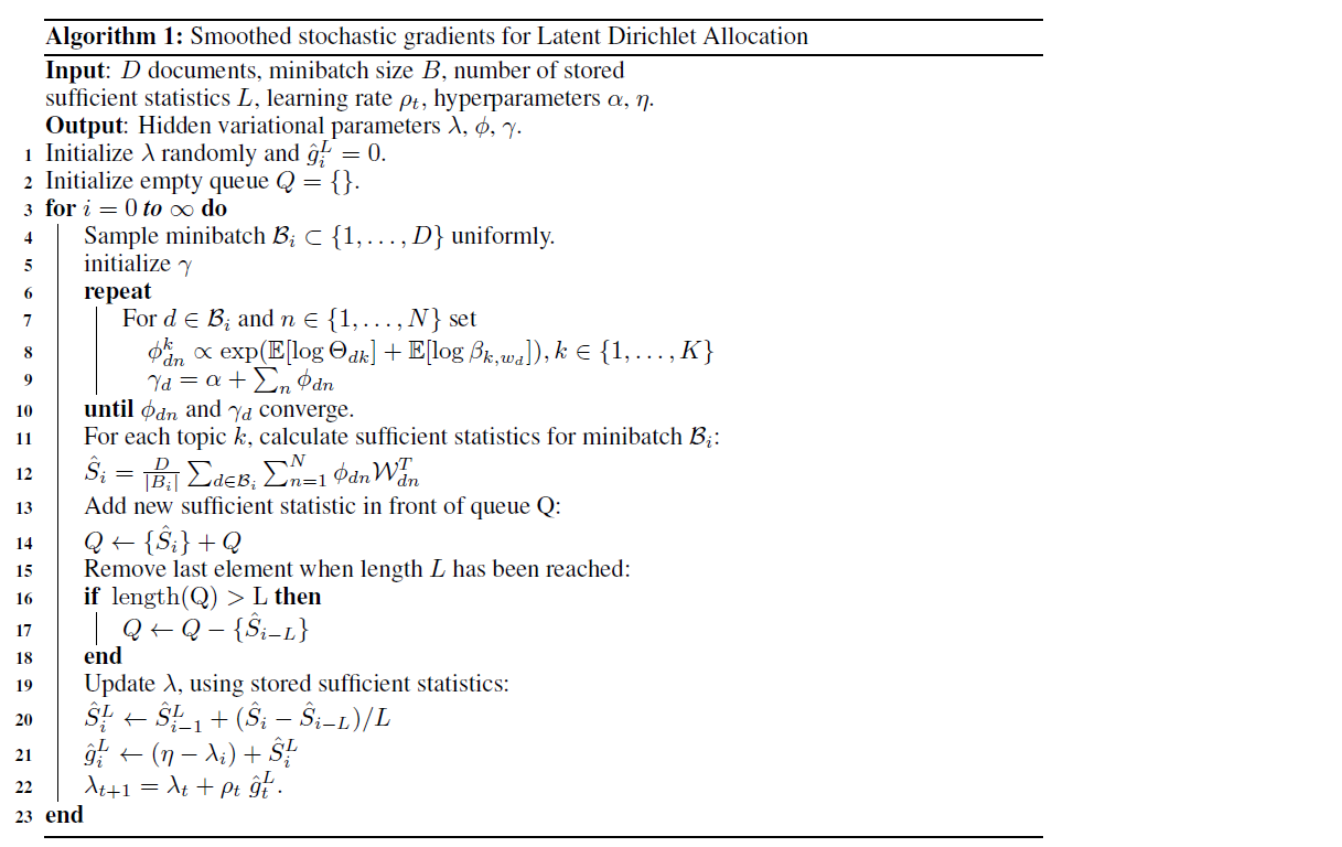
지금까지 설명한 알고리즘에 대한 자세한 pseudo-code는 다음과 같다.