MetaUAS; Universal Anomaly Segmentation with One-Prompt Meta-Learning

MetaUAS: Universal Anomaly Segmentation with One-Prompt Meta-Learning

참고: https://www.youtube.com/watch?v=1a9HV1gev9k

Contents

1. Introduction
   1. AD in Image
   2. Universal Anomaly Segmentation
   3. Mental Model
   4. One-prompt Meta Learning
2. MetaUAS
   1. Synthesizing Change Segmentation Images
   2. Overview
   3. Feature Alignment Module (FAM)
   4. Decoder
   5. Inference

1. Introduction

(1) AD in Image

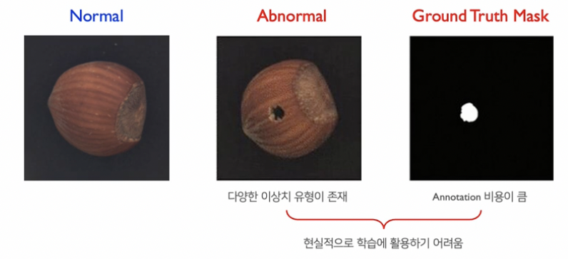
a) AC & AS

• (1) Visual anomaly classicifation (AC)
• (2) Visual anomaly segmentation (AS)
• Data: ( Normal, Abnormal, Grouth Truth Mask )

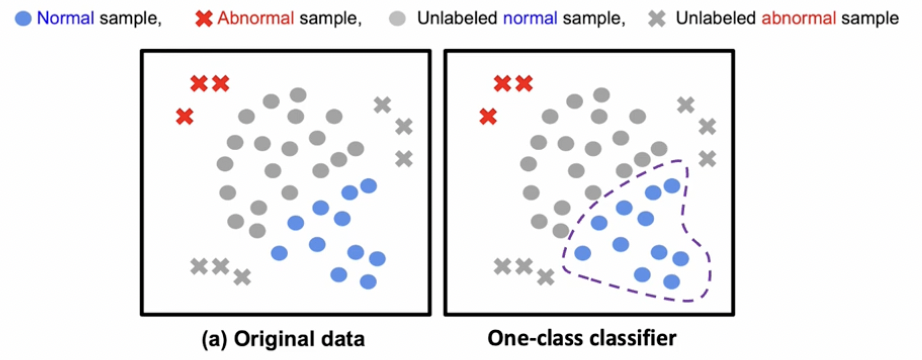
b) One-class classifier

“정상 (normal) 데이터 만”을 사용하여 구분함

c) 다양한 AD task

Training sample의 종류에 따라, 아래와 같이 4가지로 나뉠 수 있음

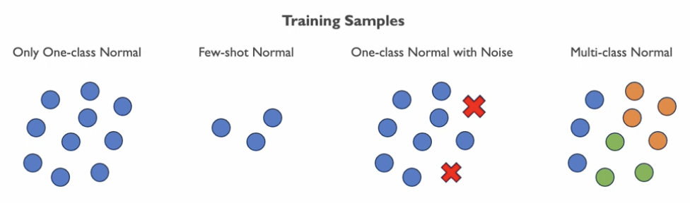
\(\rightarrow\) 기존 AD의 한계점: unseen object를 다루기 어려움

(2) Universal Anomaly Segmentation (Zero-shot AD)

최근에, LLM의 등장으로 language guidance를 활용하여 AD task의 성능을 높임.

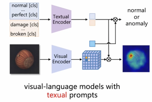
\(\rightarrow\) 그렇다면, Language guidance 없이, visual model만으로는 성능을 어디까지!?

(3) Mental Model

(Feat. 신경과학 분야)

본 논문은, Image AD를 Change segmentation 관점으로 바꾸어서 접근한다!

\(\rightarrow\) (신경 과학의) predictive coding theory

• 새로운 입력신호가 주어졌을 떄, 경험적으로 익힌 신호를 예측하고 실제 신호와 비교

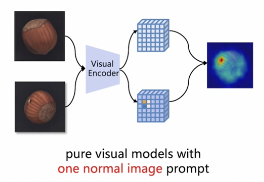
(4) One-prompt Meta Learning

One-prompt Meta Learning for Universal Anomaly Segmentation (MetaUAS)

• Change segmentation 관점으로 접근하기 위해,

  • (1) 하나의 normal prompt image

  • (2) query image

  \(\rightarrow\) (1) vs. (2) 비교를 통해 변화 여부 판단하는

2. MetaUAS

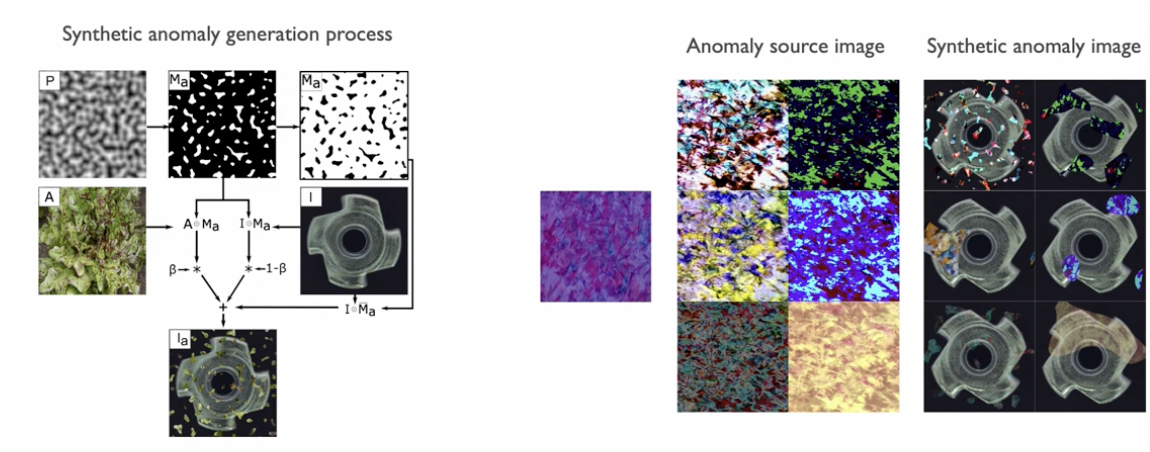
(1) Synthesizing Change Segmentation Images

AS = change segmentation의 관점!

\(\rightarrow\) 이를 위해 “새로운 데이터셋” 구성이 필요함

• 특징) “변화”가 존재하는 “두 쌍의 이미지”를 기반으로 학습

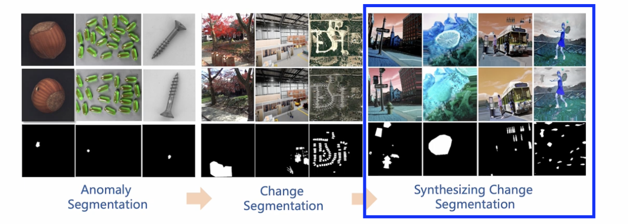
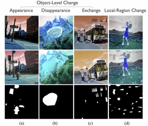
이상치 유형에 대한 정의

• (1) Object-level change

  • 1-1) Appearance
  • 1-2) Disappearance
  • 1-3) Exchange

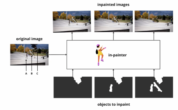
  \(\rightarrow\) “Inpainting model”을 통해 변화 생성

• (2) Local-region change

  \(\rightarrow\) “DRAEM model”을 통해 변화 생성

(1) Object-level change

(2) Local-region change

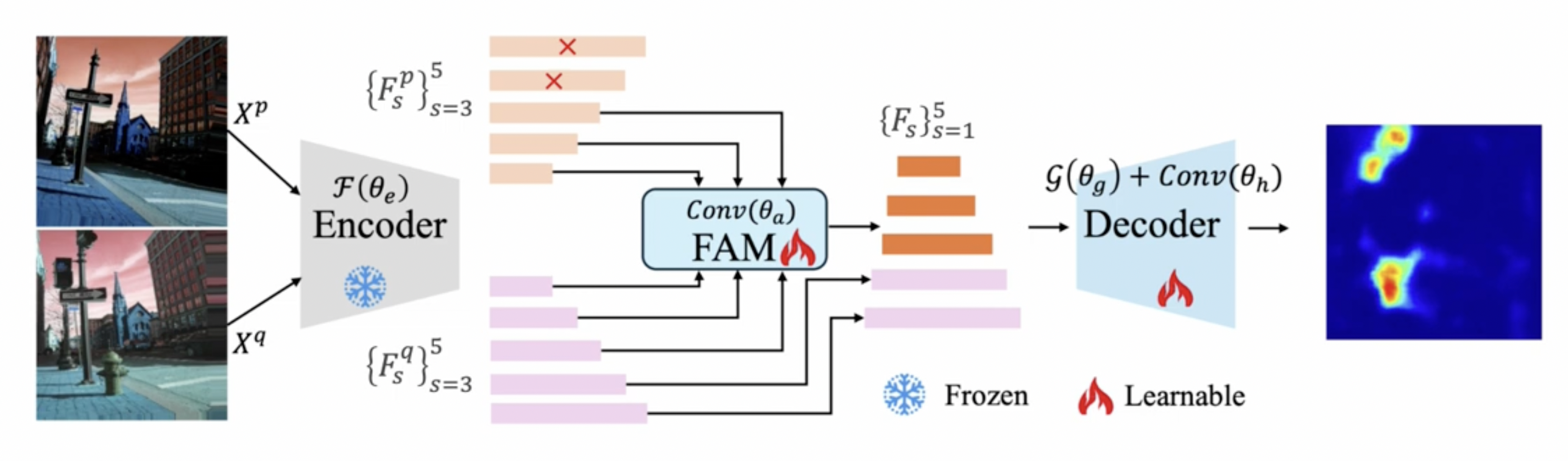
(2) Overview

Procedures

• Step 1) Dataset 구성: (query, prompt)
  • Query: 변화 탐지 대상 (\(X^q\))
  • Prompt: query와 관련된 이미지 (\(X^p\))
• Step 2) Encoder를 통해 image representation 추출
  • Stage 별 feature 추출
• Step 3) \(\{F_s^q, F_s^p\}_{s=3}^5\) (3~5번째 stage의 feature)를 FAM에 적용
  • FAM: Featuer alignment module
• Step 4) 아래의 a) & b)를 decoder에 넣어서 change segmentation
  • a) FAM의 결과
  • b) query의 low-level feature

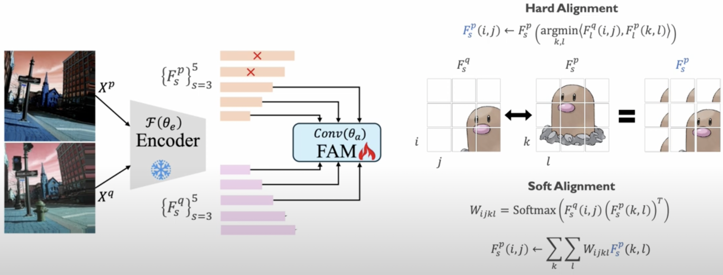
(3) Feature Alignment Module (FAM)

Details

• Soft alignment 사용
• 두 이미지의 (같은 stage의) local 정보간의 cosine simliarity를 사용하여, prompt feature 수정

\(\begin{gathered} W_{i j k l}=\operatorname{Softmax}\left(F_s^q(i, j)\left(F_s^p(k, l)\right)^T\right) \\ F_s^p(i, j) \leftarrow \sum_k \sum_l W_{i j k l} F_s^p(k, l) \end{gathered}\).

(4) Decoder

Decoder: U-Net

아래의 둘을 concat해, 최종적으로 pixel-level segmentation을 수행함

• a) FAM의 결과
• b) query의 low-level feature

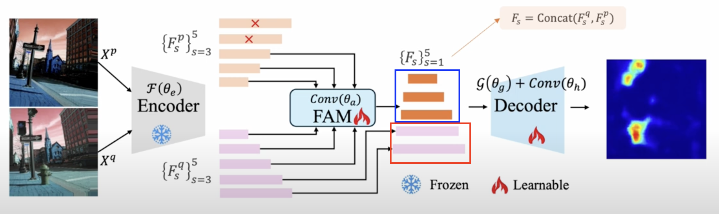
Loss function: Pixel-level binary CE loss

\(\mathcal{L}=-\sum_i\left(Y_i \cdot \log \left(\hat{Y}_i\right)+\left(1-Y_i\right) \cdot \log \left(1-\hat{Y}_i\right)\right)\).

(5) Inference

두 가지로 나뉨

• a) Class-specific query image
  • normal data 중 하나를 “랜덤”으로 선택하여 prompt image로!
• b) Class-agnostic query image
  • normal data 중 “가장 비슷한”것으로 선택하여 prompt image로!
  • class 별 normal에 대한 prompt pool 구성 후, 그 안에서 가장 비슷 (last stage feature의 cosine similarity로 비교)한 것으로 선택!