Restricted Boltzmann Machine 이론

Restricted Boltzmann Machine (RBM)

( 참고 : Hugo Larochelle의 Neural networks [5] : Restricted Boltzmann machine 강의 )

( 출처 : https://miro.medium.com/max/665/1*Z-uEtQkFPk7MtbolOSUvrA.png )

1. 개요

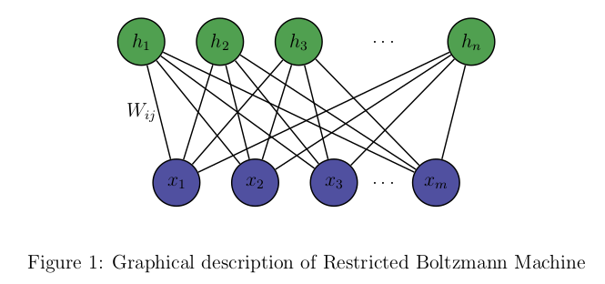
​ RBM ( Restricted Boltzmann Machine )은 위 그림과 같이 visible layer ( \(x_1, x_2, .. x_m\) ) 와 hidden layer ( \(h_1, h_2, ... , h_n\) )두 개의 layer로 구성된 모델로, 두 layer간의 연결(connection, weight)은 있지만, 같은 layer 내에서는 연결이 없게끔 제한 ( “restricted” ) 된다는 점이 특징이다. 위 그래프의 특징은, visible layer에서 hidden layer로만 연결된 dircted graph가 아니라, 서로 연결되어 있는 undirected graph라는 점이다. 여기서 모든 노드들 ( visual node \(x\) 와 hidden node \(h\))는 binary unit인 경우를 가정한다. 이 모델은 \(x\)와 \(h\)의 joint probability를 표현하여, 궁극적으로 \(p(v)\)를 최대화 하게끔 parameter의 업데이트가 이루어진다.

2. Notation

• \(h\) : hidden layer ( binary units )
• \(x\) : visible(input) layer ( binary units )
• \(w\) : weight (connection between \(h\) & \(x\))
• \(b_j\) : bias of hidden layer
• \(c_k\) : bias of visible layer
• \(j\) : number of nodes in hidden layer
• \(k\) : number of nodes in visible layer

3. Energy Function

\(x\)와 \(h\)의 joint probability는 다음과 같은 형태로 나타낼 수 있다. ( \(Z\) : normalizing constant )

\[p(x,h) = \frac{1}{Z} exp(-E(x,h))\]

위 식에서, \(E(x,h)\)를 Energy function이라 부르고, 이는 아래의 식과 같다.

\[\begin{align*} E(x,h) &= -h^{T}Wx - c^{T}x - b^{T}h \\ &= -\sum_j\sum_kW_{j,k}h_j,x_k - \sum_kc_kx_k-\sum_jb_jh_j \end{align*}\]

4. Joint distribution & Marginal Distribution

\(x\) 와 \(h\)의 joint probability 인 \(p(x,h)\)는 다음과 같이 정리할 수 있다.

\[\begin{align*} p(x,h) &= \frac{1}{Z} exp(-E(x,h))\\ &= \frac{1}{Z} exp(-h^{T}Wx - c^{T}x - b^{T}h)\\ &= \frac{1}{Z} exp(h^{T}Wx)exp(c^{T}x)exp(b^{T}h)\\ &= \frac{1}{Z} \prod_j\prod_k exp(W_{j,k}h_jx_k)\prod_k exp(c_kx_k)\prod_j exp(b_jh_j) \end{align*}\]

위에서 구한 \(p(x,h)\)를 marginalize하면 다음과 같다.

\[\begin{align*} p(x) &= \sum_{h\in \{0,1\}}p(x,h) \\ &= \frac{1}{Z}\sum_{h\in \{0,1\}} exp(-E(x,h)) \\ &= \frac{1}{Z}exp(c^{T}x + \sum_{j=1}^{H}log(1+exp(b_j + W_j\cdot x)))\\ &= \frac{1}{Z}exp(-F(x)) \end{align*}\]

( \(F(x)\) 는 free energy라고 부른다 )

5. Inference 과정

( derivation은 생략 )

• [1] given \(x\), predict \(h\)

  \[p(h\mid x) = \prod_jp(h_j\mid x)\] \[\begin{align*} p(h_j = 1 \mid x) &= \frac{1}{1+exp(-(b_j+W_j\cdot x))}\\ &= sigmoid(b_j + W_j\cdot x) \end{align*}\]

• [2] given \(h\), predict \(x\)

  \[p(x\mid h) = \prod_kp(x_k\mid h)\] \[\begin{align*} p(x_k = 1 \mid h) &= \frac{1}{1+exp(-(c_k+ h^{T}W_k))}\\ &= sigmoid(c_k + h^{T}W_k) \end{align*}\]

6. Minimizing Cost Function

RBM을 학습시키기 위해, 우리는 다음의 cost function (NLL, negative log-likelihood)을 최소화해야한다.

\[\frac{1}{T} \sum_t l(f(x^{(t)})) = \frac{1}{T}\sum_t -logp(x^{(t)})\]

Gradient Descent를 통해 weight를 업데이트 해나갈 것이다.

\(-logp(x^{(t)})\)를 \(\theta\) (파라미터들)로 미분을 하면,

다음과 같이 positive phase와 negative phase로 나눌 수 있다.

\[\frac{\partial -logp(x^{(t)}))}{\partial \theta } = E_h[\frac{\partial E(x^{(t)},h)}{\partial \theta}\mid x^{(t)}] - E_{x,h}[\frac{\partial E(x,h)}{\partial \theta}]\]

• positive phase (각각의 observation \(x^{(t)}\)에 의존하는 부분) : \(E_h[\frac{\partial E(x^{(t)},h)}{\partial \theta}\mid x^{(t)}]\)
• negative phase (오직 우리의 모델에만 의존하는 부분) : \(E_{x,h}[\frac{\partial E(x,h)}{\partial \theta}]\)

우리는 positive phase를 줄이는 방향으로, negative phase를 키우는 방향으로 파라미터들을 업데이트 해나가야 한다.

7. Contrastive Divergence

​ 위의 6.Training RBM에서 구한 negative phase인 \(E_{x,h}[\frac{\partial E(x,h)}{\partial \theta}]\)은 계산하기가 쉽지 않다. (가능한 \(x\)와 \(h\)의 모든 조합을 고려해야 하므로 ) 이를 해결하기 위해 사용하는 것이 바로 Contrastive Divergence이다. 이 알고리즘을 요약하면, \(p(x,h)\)를 converge할때까지 Gibbs sampling을 하는 것이 아니라, 딱 한번만 돌려서 이를 근사하는 것을 의미한다. 이를 한번이 아닌 k번하게 되면, 이를 Contrastive Divergence-k (CD-k)라고 한다.

위 그림을 통해 쉽게 이해할 수 있을 것이다. \(x^{(t)}\)를 시작으로, hidden layer-visible layer-hidden layer-visible layer-….를 반복하면서 weight를 업데이트한다.

( \(\tilde{x}\) : 깁스 샘플링을 통해 얻어낸 negative sample of \(x\) )

( \(\tilde{h}\) : 깁스 샘플링을 통해 얻어낸 negative sample of \(h\) )

positive phase와 negative phase를 각각 아래과 같이 근사할 수 있다. 또한, 아래의 그래프에서 알 수 있듯, \(E(x,h)\)값이 \((x^{(t)},\tilde{h}^{(t)})\)에서는 낮게, \((\tilde{x} , \tilde{h})\)에서는 높게끔 만들어야 한다. ( \(p(x,h)\)에서는 반대로 )

8. Update Weights

\[\begin{align*} \frac{\partial E(x,h)}{\partial W_{jk} } &= \frac{\partial }{\partial W_{jk} }(-\sum_j\sum_kW_{j,k}h_j,x_k - \sum_kc_kx_k-\sum_jb_jh_j )\\ &= \frac{\partial }{\partial W_{jk} }(-\sum_j\sum_kW_{j,k}h_j,x_k )\\ &= -h_jx_k \end{align*}\] \[\begin{align*} E_h[\frac{\partial E(x,h)}{\partial W_{jk} }\mid x] &= E_h[-h_jx_k \mid x] \\ &= \sum_{h_j \in \{0,1\}}-h_jx_kp(h_j \mid x)\\ &= -x_k p(h_j=1 \mid x) \end{align*}\]

let \(h(x) = sigmoid(b+Wx)\)

따라서, \(E(x,h)\)를 weight \(w\)에 대해 미분한 값은 다음과 같이 정리할 수 있다.

\[E_h[\bigtriangledown _w E(x,h)\mid x] = -h(x) x^{T}\]

Update Rules

위 식을 끝으로, 이제 \(w\)를 update하기 위한 준비는 모두 끝났다. update rule은 아래와 같다.

\[\begin{align*} W &\leftarrow W- \alpha (\bigtriangledown_w(-logp(x^{(t)})))\\ &\leftarrow W- \alpha(E_h[\bigtriangledown_w E(x^{(t)},h) \mid x^{(t)}] - E_{x,h}[\bigtriangledown_w E(x,h)])\\ &\leftarrow W- \alpha(E_h[\bigtriangledown_w E(x^{(t)},h) \mid x^{(t)}] - E_{x,h}[\bigtriangledown_w E(\tilde{x},h) \mid \tilde{x}])\\ &\leftarrow W+ \alpha(h(x^{(t)}){x^{(t)}}^{T}-h(\tilde{x})\tilde{x}^T) \end{align*}\]

9. Summary of RBM

RBM의 CD ( Contrastive Divergence) - K의 알고리즘은 아래와 같다

• 각각의 training data \(x(t)\)에 대해,
  • k-step Gibbs sampling을 사용하여 negative sample \(\tilde{x}\)를 샘플링한다
  • 파라미터를 업데이트 한다
    • \[W \leftarrow W+ \alpha(h(x^{(t)}){x^{(t)}}^{T}-h(\tilde{x})\tilde{x}^T)\]
    • \[b \leftarrow b + \alpha(h(x^{(t)})-h(\tilde{x}))\]
    • \[c \leftarrow c + \alpha(x^{(t)}-\tilde{x})\]
• Stopping Criteria에 도달하기 전까지 위 과정을 반복한다.