30.(paper) 1.Efficient Estimation of Word Representations in Vector Space

1.Efficient Estimation of Word Representations in Vector Space (2013)

목차

1. Abstract
2. Introduction

3. Model Architectures

   1. NNLM ( Feedforward NNLM )
   2. RNNLM ( Recurrent NNLM )
4. New Log-Linear Models
   1. CBOW
   2. Skip-gram

Abstract

Word2Vec : (1) Skip-gram & (2) CBOW

• able to capture the similarity of words
• improvement in accuracy & speed

1. Introduction

Previous models : N-gram … similarity (X) & use indices (O)

Proposes “distributed representations of words”

( \(\leftrightarrow\) previous ones were “SPARSE” representation….one-hot encoded vector )

2. Model Architectures

This paper focuses on “distributed representations” of words, learned by NN

Training Complexity : \(O=E \times T \times Q\)

• \(E\) : training epoch
• \(T\) : number of words
• \(Q\) : (defined further for each model architecture)

use SGD & BP

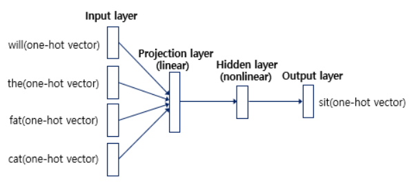
2-1. NNLM (Feedforward NNLM)

consists of 1) input, 2) projection, 3) hidden, 4) output layers

1) Input layer

• \(N\) words are one-hot encoded ( = 1-of-V coding )

2) Projection layer

• dimension : \(N \times D\)
• shared projection matrix

3) Hidden layer

• projection-hidden layer : complex computation

  ( since values in projection layer are dense )

• compute “probability distribution” over all the words in vocabulary

4) Output layer

• dimension : \(V\)

Time complexity : \(Q=(N\times D) + (N\times D \times H) + (H \times V)\)

• last term \((H \times V)\) is the dominating term

  \(\rightarrow\) use Negative Sampling, Hierarchical softmax to reduce this!

  \(\rightarrow\) from \(V\) to \(\log_2V\)

2-2. RNNLM (Recurrent NNLM)

overcome limitation of NNLM ( = need to specify context length, N )

RNN :

• input, hidden, output layer (no projection layer)

• information from past can be represented by “hidden layer state” \(h_t\)

  ( updated by \(x_t\) and \(h_{t-1}\) )

Time complexity : \(Q=(H\times H) + (H \times V)\)

• last term \((H \times V)\) is the dominating term

  \(\rightarrow\) use Negative Sampling, Hierarchical softmax to reduce this!

  \(\rightarrow\) from \(V\) to \(\log_2V\)

3. New Log-Linear Models

propose 2 models, (1) CBOW & (2) Skip-gram

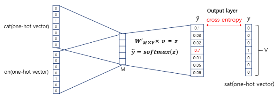
3-1. CBOW

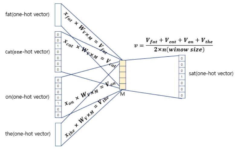
\(Q = (N \times D) + (D \times \log_2(V))\).

3-2. Skip-gram

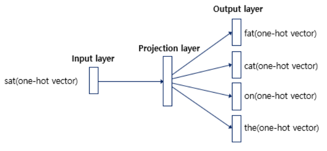
\(Q = C \times (D + D \times \log_2(V))\).