[Paper Review] 20. Seeing what a GAN cannot generate
Contents
- Abstract
- Introduction
- Method
- Quantifying distribution-level model collapse
- Quantifying instance-level mode collapse
0. Abstract
GAN training’s key issue : mode collapse
- little work have focused on “understanding & quantifying mode collapse”
\(\rightarrow\) visualize mode collapse at both..
- 1) distribution level
- 2) instance level
1. Introduction
this paper aims to provide insights about dropped modes
( not to measure GAN quality using single number )
Particularly, wish to know…
- Does GAN deviate from target distn, by ignoring difficult images altogether?
- are there specific, semantically meaningful parts and objects that a GAN decides not to learn?
2. Method
goal : visualize & understand the semantic concepts that GAN “CAN NOT” generate
( in both (1) distn & (2) image instance )
Proceed in 2 steps!
[Step 1] Generated Image Segmentation
-
segment both “1) generated” & “2) target” images
-
identify types of object that generator omits
( compared to distn of real images )
[Step 2] Layer Inversion
- visualize HOW the dropped object classes are omitted for individual images
(1) Quantifying distribution-level model collapse
errors of GAN :
-
analyzed by exploiting “hierarchical structure” of scene image
-
each scene = natural decomposition into objects
\(\rightarrow\) we can estimate deviations from true distn of scenes
Example)
GAN that render bedrooms, should also render some curtains
-
if curtain statistics depart from true image,
we will know we can look at curtains to see a specific flaw in GAN
use segmentation using Unified Perceptual Parsing Network
( labels each pixel with 336 object classes)
Figure 2

- visualization of mean statistics for 2 networks
- mean segmentation frequencuy
- network1 vs true distn
- network2 vs true distn
Possible to summarize statistical differences in segmentation in a single number
- FSD (Frechet Segmentation Distance)
[ Conclusion ]
-
Generated Image Segmentation Statistics measure the entire distn
-
BUT, do not single out specific images,
where an object should have been generated, but was not!
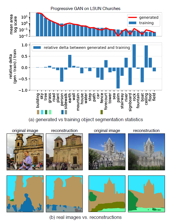
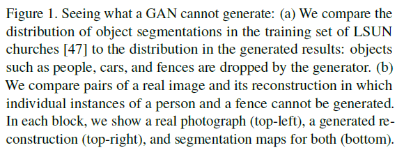
(2) Quantifying instance-level mode collapse
compare image pairs \((\mathbf{x},\mathbf{x}^{'})\)
-
\(\mathbf{x}\) : real image
( have particular object, which is NOT in GENERATED image )
-
\(\mathbf{x}^{'}\) : projection onto space of all images
( output of GAN, where input is \(z^{'}\) )
Tractable Inversion Problem
seek \(\mathrm{x}^{\prime}=G\left(\mathbf{z}^{*}\right)\)
-
where \(\mathrm{z}^{*}=\arg \min _{\mathrm{z}} \ell(G(\mathbf{z}), \mathrm{x})\)
-
but, fail to solve this inversion! ( due to many layers in \(G\) )
therefore, solve a tractable subproblem of full inversion
\(\rightarrow\) decompose \(G\) !
Decomposition of \(G\)
-
\(G=G_{f}\left(g_{n}\left(\cdots\left(\left(g_{1}(\mathbf{z})\right)\right)\right)\right.\).
-
thus, \(\operatorname{range}(G) \subset \operatorname{range}\left(G_{f}\right)\)
-
meaning : any image that can not be generated by \(G_f\) ,
can not be generated by \(G\) either
-
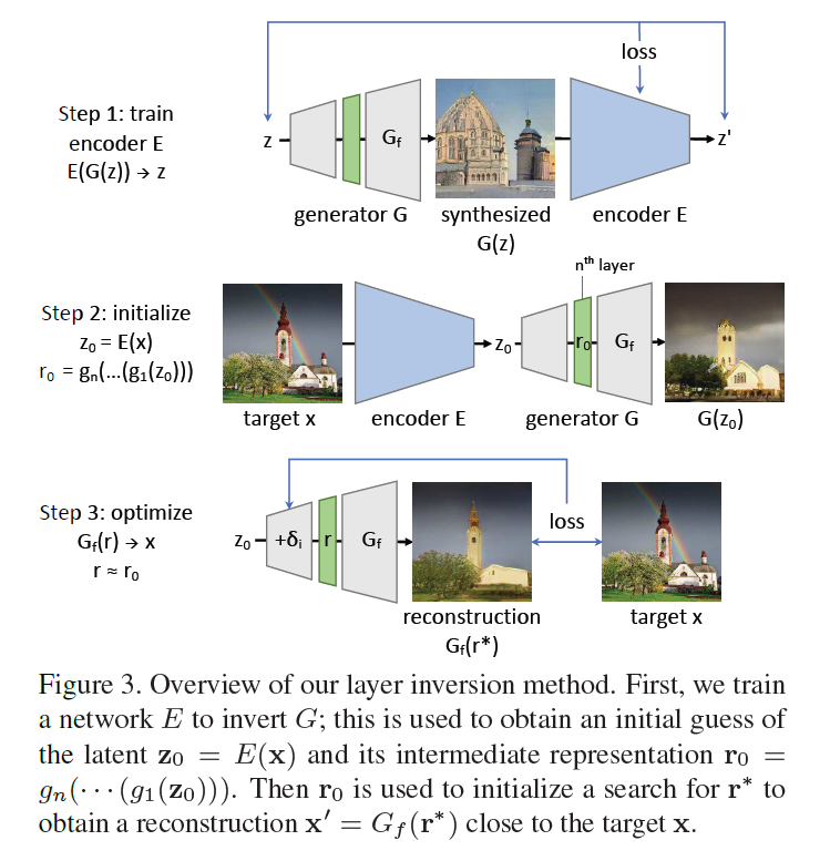
Layer Inversion
-
goal : visualize omissions
-
by solving easier problem of inverting the later layers \(G_f\)
-
\(\mathrm{x}^{\prime}=G_{f}\left(\mathrm{r}^{*}\right)\),
where \(\mathbf{r}^{*}=\underset{\mathbf{r}}{\arg \min } \ell\left(G_{f}(\mathbf{r}), \mathbf{x}\right)\)
-
-
solve in 2 steps
-
step 1) construct (NN) \(E\), that approximately inverts entire \(G\)
& compute an estimate \(\mathbf{z}_{0}=E(\mathbf{x})\)
-
step 2) identify an intermediate representation
\(\mathbf{r}^{*} \approx \mathbf{r}_{0}=g_{n}\left(\cdots\left(g_{1}\left(\mathbf{z}_{0}\right)\right)\right)\).
where \(G_{f}\left(\mathbf{r}^{*}\right)\) closely recover \(x\)
-
Layer-wise Network Inversion
train a small network \(e_i\) to (approximately) invert \(g_i\)
-
train to minimize both left & right inversion losses
\(\begin{aligned} \mathcal{L}_{\mathrm{L}} & \equiv \mathbb{E}_{\mathbf{Z}}\left[ \mid \mid \mathbf{r}_{i-1}-e\left(g_{i}\left(\mathbf{r}_{i-1}\right)\right) \mid \mid _{1}\right] \\ \mathcal{L}_{\mathrm{R}} & \equiv \mathbb{E}_{\mathbf{Z}}\left[ \mid \mid \mathbf{r}_{i}-g_{i}\left(e\left(\mathbf{r}_{i}\right)\right) \mid \mid _{1}\right] \\ e_{i} &=\underset{e}{\arg \min } \quad \mathcal{L}_{\mathrm{L}}+\lambda_{\mathrm{R}} \mathcal{L}_{\mathrm{R}} \end{aligned}\).
once layers are all inverted…
compose an inversion network for entire \(G\)!
- \(E^{*}=e_{1}\left(e_{2}\left(\cdots\left(e_{n}\left(e_{f}(\mathrm{x})\right)\right)\right)\right)\).
Layer-wise image optimization
inverting entire \(G\) is difficult ( mentioned above )
Thus, start from…
-
1) \(\mathbf{r}_{0}=g_{n}\left(\cdots\left(g_{1}\left(\mathbf{z}_{0}\right)\right)\right)\)
-
2) seek an intermediate representation \(\mathrm{r}^{*}\)
- where \(G_{f}\left(\mathrm{r}^{*}\right)\) becomes reconstructed image
-
(summary)
\(\begin{aligned} \mathbf{z}_{0} & \equiv E(\mathbf{x}) \\ \mathrm{r} & \equiv \delta_{n}+g_{n}\left(\cdots\left(\delta_{2}+g_{2}\left(\delta_{1}+g_{1}\left(\mathbf{z}_{0}\right)\right)\right)\right) \\ \mathbf{r}^{*} &=\underset{\mathbf{r}}{\arg \min }\left(\ell\left(\mathrm{x}, G_{f}(\mathrm{r})\right)+\lambda_{\mathrm{reg}} \sum_{i} \mid \mid \delta_{i} \mid \mid ^{2}\right) \end{aligned}\).
- begin with initial guess \(\mathbf{z}_{0}\)
- then learn small perturbations of each layer