[Paper Review] 27.(i2i translation) Toward Multimodal Image-to-Image Translation

[Paper Review] 27. Toward Multimodal Image-to-Image Translation

Contents

1. Abstract
2. Introduction
3. Related Work
   1. Image-to-Image Translation
   2. Unpaired Image-to-Image Translation
   3. Cycle Consistency
   4. Neural Style Transfer
4. Formulation
   1. Adversarial Loss
   2. Cycle Consistency Loss
   3. Full Objective

0. Abstract

single input image may correspond to MULTIPLE possible outputs

\(\rightarrow\) aim to model a distribution of possible outputs in a conditional generative modeling setting

1. Introduction

common problem in existing methods : mode collapse

• this paper solves this!

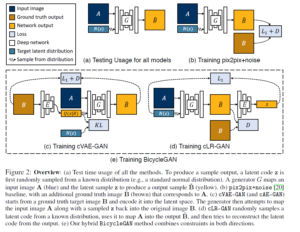
Starts with pix2pix framework

• trains a \(G\), conditioned on the input image, with 2 losses
  • 1) regression loss : to produce similar output to the known paired ground truth image
  • 2) learned discriminator loss : to encourage realism

propose encouraging a bijection between the output & latent space

Explore several objective functions!

• 1) cVAE-GAN ( Conditional Variational Autoencoder GAN)
  • encoding the “ground truth image” to “latent space”
  • along with “input image”, the generator should be able to reconstruct the specific output image
• 2) cLR-GAN ( Conditional Latent Regressor GAN )
  • first, provide a randomly drawn latent vector
  • encoder then attempts to recover the latent vector from the output image
• 3) BicycleGAN
  • combine 1) & 2)

2. Related Works

3. Multimodal Image-to-Image Translation

Goal : learn a multi-modal mapping, between 2 image domains

• input domain : \(\mathcal{A} \subset \mathrm{R}^{H \times W \times 3}\)

• output domain : \(\mathcal{B} \subset \mathbb{R}^{H \times W \times 3}\)

• given a dataset of paired instances from these domains

  ( = representative of joint dinst \(p(A,B)\) )

• should be able to generate a diverse set of output \(\widehat{B}\) ‘s

( first discuss a simple extension of existing methods )

1) Baseline : pix2pix + noise ( \(z \rightarrow \hat{\mathbf{B}}\) )

• conditional adversarial networks
• randomly drawn noise \(z\) is added for stochasticity
• Loss Function :
  • 1) \(\mathcal{L}_{\mathrm{GAN}}(G, D)=\mathbb{E}_{\mathbf{A}, \mathbf{B} \sim p(\mathbf{A}, \mathbf{B})}[\log (D(\mathbf{A}, \mathbf{B}))]+\mathbb{E}_{\mathbf{A} \sim p(\mathbf{A}), \mathbf{z} \sim p(\mathbf{z})}[\log (1-D(\mathbf{A}, G(\mathbf{A}, \mathbf{z})))]\).
  • 2) \(\mathcal{L}_{1}^{\text {image }}(G)=\mathbb{E}_{\mathbf{A}, \mathbf{B} \sim p(\mathbf{A}, \mathbf{B}), \mathbf{z} \sim p(\mathbf{z})} \mid \mid \mathbf{B}-G(\mathbf{A}, \mathbf{z}) \mid \mid _{1}\).
• Final Loss Function :
  • \(G^{*}=\arg \min _{G} \max _{D} \quad \mathcal{L}_{\mathrm{GAN}}(G, D)+\lambda \mathcal{L}_{1}^{\mathrm{image}}(G)\).

2) Conditional Variational Autoencoder GAN : cVAE-GAN \((\mathrm{B} \rightarrow \mathrm{z} \rightarrow \widehat{\mathrm{B}})\)

• one way to force \(z\) to be “useful” :
  • directly map ground truth \(B\) to \(z\), using encoding function \(E\)
• \(G\) uses both (1) latent code & (2) input image \(A\)
  • to make a desired output \(\hat{\mathbf{B}}\)
• Loss Function
  • 1) \(\mathcal{L}_{\mathrm{GAN}}^{\mathrm{VAE}}=\mathbb{E}_{\mathbf{A}, \mathbf{B} \sim p(\mathbf{A}, \mathbf{B})}[\log (D(\mathbf{A}, \mathbf{B}))]+\mathbb{E}_{\mathbf{A}, \mathbf{B} \sim p(\mathbf{A}, \mathbf{B}), \mathbf{z} \sim E(\mathbf{B})}[\log (1-D(\mathbf{A}, G(\mathbf{A}, \mathbf{z})))]\).
  • 2) \(\mathcal{L}_{1}^{\mathrm{VAE}}(G)=\mathbb{E}_{\mathbf{A}, \mathbf{B} \sim p(\mathbf{A}, \mathbf{B}), \mathbf{z} \sim E(\mathbf{B})} \mid \mid \mathbf{B}-G(\mathbf{A}, \mathbf{z}) \mid \mid _{1}\).
  • 3) \(\mathcal{L}_{\mathrm{KL}}(E)=\mathbb{E}_{\mathbf{B} \sim p(\mathbf{B})}\left[\mathcal{D}_{\mathrm{KL}}(E(\mathbf{B}) \mid \mid \mathcal{N}(0, I))\right]\).
• Final Loss Function :
  • \(G^{*}, E^{*}=\arg \min _{G, E} \max _{D} \quad \mathcal{L}_{\mathrm{GAN}}^{\mathrm{VAE}}(G, D, E)+\lambda \mathcal{L}_{1}^{\mathrm{VAE}}(G, E)+\lambda_{\mathrm{KL}} \mathcal{L}_{\mathrm{KL}}(E)\).

3) Conditional Latent Regressor GAN : cLR-GAN \((\mathbf{z} \rightarrow \widehat{\mathbf{B}} \rightarrow \widehat{\mathbf{Z}})\)

• enforce \(G\) to use \(z\), while staying close to the actual test time distn \(p(z)\)
• Loss Function
  • 1) \(\mathcal{L}_{\mathrm{GAN}}(G, D)=\mathbb{E}_{\mathbf{A}, \mathbf{B} \sim p(\mathbf{A}, \mathbf{B})}[\log (D(\mathbf{A}, \mathbf{B}))]+\mathbb{E}_{\mathbf{A} \sim p(\mathbf{A}), \mathbf{z} \sim p(\mathbf{z})}[\log (1-D(\mathbf{A}, G(\mathbf{A}, \mathbf{z})))]\).
  • 2) \(\mathcal{L}_{1}^{\text {latent }}(G, E)=\mathbb{E}_{\mathbf{A} \sim p(\mathbf{A}), \mathbf{z} \sim p(\mathbf{z})} \mid \mid \mathbf{z}-E(G(\mathbf{A}, \mathbf{z})) \mid \mid _{1}\)
• Final Loss Function :
  • \(G^{*}, E^{*}=\arg \min _{G, E} \max _{D} \quad \mathcal{L}_{\mathrm{GAN}}(G, D)+\lambda_{\text {latent }} \mathcal{L}_{1}^{\text {latent }}(G, E)\).

4) Our Hybrid Model : BicycleGAN

combine “cVAE-GAN” & “cLR-GAN” objectives!

\(\begin{aligned} G^{*}, E^{*}=\arg \min _{G, E} \max _{D} & \mathcal{L}_{\mathrm{GAN}}^{\mathrm{VAE}}(G, D, E)+\lambda \mathcal{L}_{1}^{\mathrm{VAE}}(G, E) \\ &+\mathcal{L}_{\mathrm{GAN}}(G, D)+\lambda_{\text {latent }} \mathcal{L}_{1}^{\text {latent }}(G, E)+\lambda_{\mathrm{KL}} \mathcal{L}_{\mathrm{KL}}(E) \end{aligned}\).