[ 10. Knowledge Graph Embeddings ]
( 참고 : CS224W: Machine Learning with Graphs )
Contents
- 10-1. RGCN (Relational GCN)
- 10-2. Knowledge Graphs
- 10-3. Knowledge Graph Completion
Heterogeneous Graphs
will extend “one edge” type to “multiple edge” types
Heterogeneous graphs
- \(\boldsymbol{G}=(\boldsymbol{V}, \boldsymbol{E}, \boldsymbol{R}, \boldsymbol{T})\).
- 1) NODES with node types : \(v_{i} \in V\)
- 2) EDGES with relation types : \(\left(v_{i}, r, v_{j}\right) \in E\)
- 3) NODE TYPE : \(T\left(v_{i}\right)\)
- 4) RELATION TYPE : \(r \in R\)
Heterogeneous graphs models :
- 1) Relational GCNs
- 2) Knowledge Graphs
- 3) Embeddings for KG Completion
10-1. RGCN (Relational GCN)
Heterogeneous graphs
- multiple edges
- multiple relation types
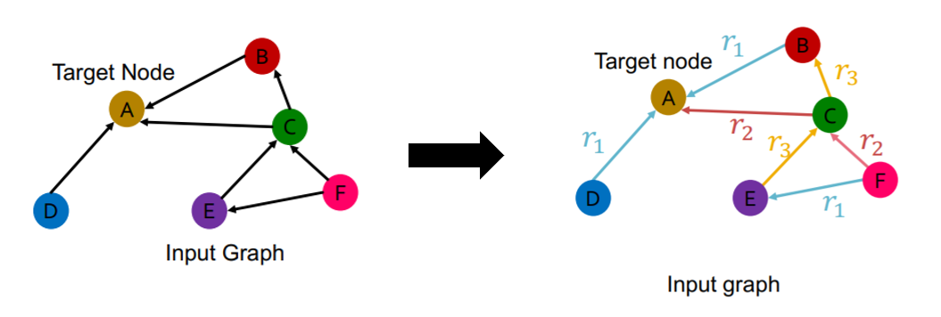
Solution :
- use different NN for different relation types
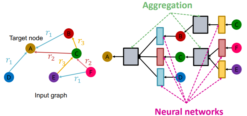
Relational GCN :
\(\mathbf{h}_{v}^{(l+1)}=\sigma\left(\sum_{r \in R} \sum_{u \in N_{v}^{r}} \frac{1}{c_{v, r}} \mathbf{W}_{r}^{(l)} \mathbf{h}_{u}^{(l)}+\mathbf{W}_{0}^{(l)} \mathbf{h}_{v}^{(l)}\right)\).
- where \(c_{v, r}=\mid N_{v}^{r} \mid\)
decompose as “Message + Aggregation”
- 1) Message :
- 1-1) neighbor : \(\mathbf{m}_{u, r}^{(l)}=\frac{1}{c_{v, r}} \mathbf{W}_{r}^{(l)} \mathbf{h}_{u}^{(l)}\).
- 1-2) self loop : \(\mathbf{m}_{v}^{(l)}=\mathbf{W}_{0}^{(l)} \mathbf{h}_{v}^{(l)}\).
- 2) Aggregation :
- \(\mathbf{h}_{v}^{(l+1)}=\sigma\left(\operatorname{Sum}\left(\left\{\mathbf{m}_{u, r}^{(l)}, u \in N(v)\right\} \cup\left\{\mathbf{m}_{v}^{(l)}\right\}\right)\right)\).
Scalability of RGCN
-
number of layers : \(L\)
-
each relation has \(L\) matrices : \(\mathbf{W}_{r}^{(1)}, \mathbf{W}_{r}^{(2)} \cdots \mathbf{W}_{r}^{(L)}\)
-
dimension of \(\mathbf{W}_{r}^{(l)}\) is \(d^{(l+1)} \times d^{(l)}\)
-
overfitting issue! how to solve?
-
-
solution : regularize \(\mathbf{W}_{r}^{(l)}\)
- 1) block diagonal matrices
- 2) basis/dictionary learning
(1) Block Diagonal Matrices
Use block diagonal matrices for \(\mathbf{W}_{r}^{}\)
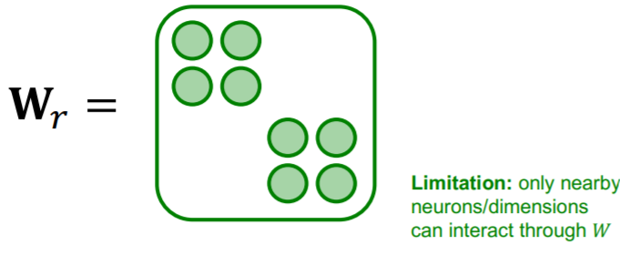
if we use \(B\) low-dim matrices… number of params will becom
- before ) \(d^{(l+1)} \times d^{(l)}\)
- after ) \(B \times \frac{d^{(l+1)}}{B} \times \frac{d^{(l)}}{B}\)
(2) Basis Learning
Share weights across different relations!
Matrix = “linear combination” of “basis” transformation
-
\(\mathbf{W}_{r}=\sum_{b=1}^{B} a_{r b} \cdot \mathbf{V}_{b}\).
- \(\mathbf{V}_{b}\) : basis matrices ( shared across all relations )
-
\(a_{r b}\) : importance weight of matrix \(\mathbf{V}_{b}\)
- \(B\) : number of basis to use
-
thus, only need to learn \(\left\{a_{r b}\right\}_{b=1}^{B}\)
(3) Example : Node Classification
-
goal : predict the class of node \(A\), from \(k\) classes
-
final layer (prediction head) :
\(\mathbf{h}_{A}^{(L)} \in \mathbb{R}^{k}\) = probability of each classes
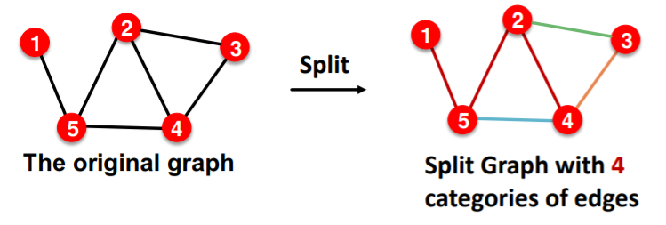
(4) Example : Link Prediction
Stratified Split….with 4 categories of edges
- 1-1) [TRAIN] message edges
- 1-2) [TRAIN] supervision edges
- 2) [VALIDATION] edges
- 3) [TEST] edges
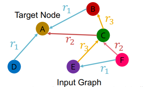
Example )
-
training message edges : all others
-
training supervision edge : (\(E , r_3, A\) )
\(\rightarrow\) score this edge
- final layer of \(E\) : \(\mathbf{h}_{E}^{(L)}\)
-
final layer of \(A\) : \(\mathbf{h}_{A}^{(L)}\)
-
score function : \(f_{r}: \mathbb{R}^{d} \times \mathbb{R}^{d} \rightarrow \mathbb{R}\)
-
final score
= \(f_{r_{1}}\left(\mathbf{h}_{E}, \mathbf{h}_{A}\right)=\mathbf{h}_{E}^{T} \mathbf{W}_{r_{1}} \mathbf{h}_{A}, \mathbf{W}_{r_{1}} \in \mathbb{R}^{d \times d}\)
Training Procedure :
step 1) use RGCN to score “training supervision edge”
- ex) \(\left(E, r_{3}, A\right)\)
step 2) create negative edge by perturbing supervision edge
- ex) \(\left(E, r_{3}, B\right), \left(E, r_{3}, D\right)\)
- note that negative edges should also NOT BELONG to TRAINING MESSAGE EDGES!
step 3) use GNN model to score negative edges
step 4) optimize CE loss
-
\[\ell=-\log \sigma\left(f_{r_{3}}\left(h_{E}, h_{A}\right)\right)-\log \left(1-\sigma\left(f_{r_{3}}\left(h_{E}, h_{B}\right)\right)\right)\]
- (1) maximize “training supervision edge”
- (2) minimize “negative edge”
Evaluation Procedure
Example :
-
validation edge : \((E,r_3,D)\)
-
score of “validation edge” should be higher than
\((E,r_3,v)\) , where it is NOT in the training message/supervision edges
Procedure :
step 1) calculate the score of \((E,r_3,D)\)
step 2) calculate score of all negative edges \(\left\{\left(E, r_{3}, v\right) \mid v \in\{B, F\}\right\}\)
step 3) obtain ranking (RK) of \((E,r_3,D)\)
step 4) calculate metrics
- 1) Hits@k = \(1[RK \neq k]\)
- 2) Reciprocal Rank = \(1/RK\)
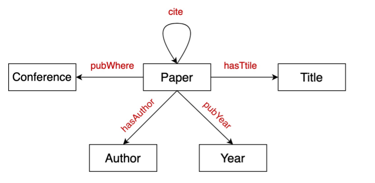
10-2. Knowledge Graphs
Knowledge in graph form
- nodes : ENTITIES
- label of nodes : TYPES
- edges : RELATIONSHIPS
KG(Knowledge Graph) is an example of heterogeneous graph
Example )
10-3. Knowledge Graph Completion
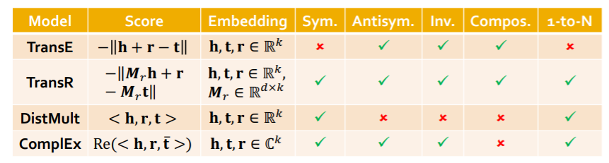
Models
- 1) TransE
- 2) TransR
- 3) DistMul
- 4) ComplEx
(1) KG Completion Task
task : for a given (HEAD, RELATION), predict “missing tails”
Example )
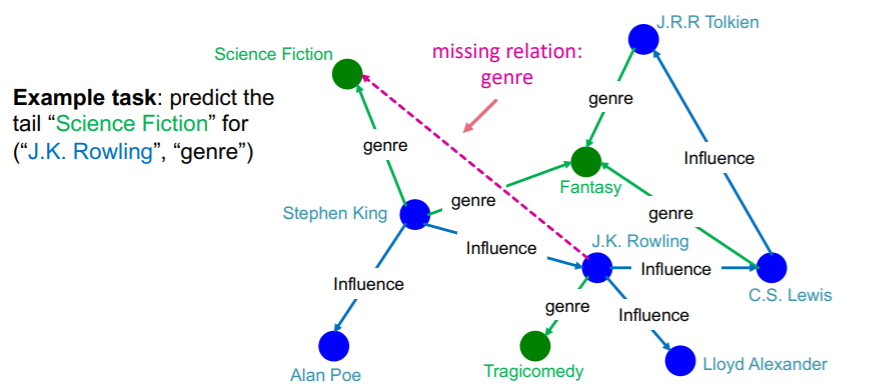
Notation
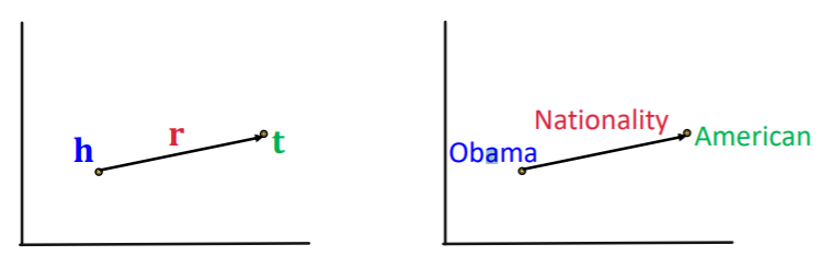
- edges are represented as triples \((h,r,t)\)
- \(h\) : head
- \(r\) : relation
- \(t\) : tail
- given \((h,r,t)\), make embedding \((h,r)\) to be close to embedding \(t\)
- Q1) how to embed?
- Q2) how to define closeness?
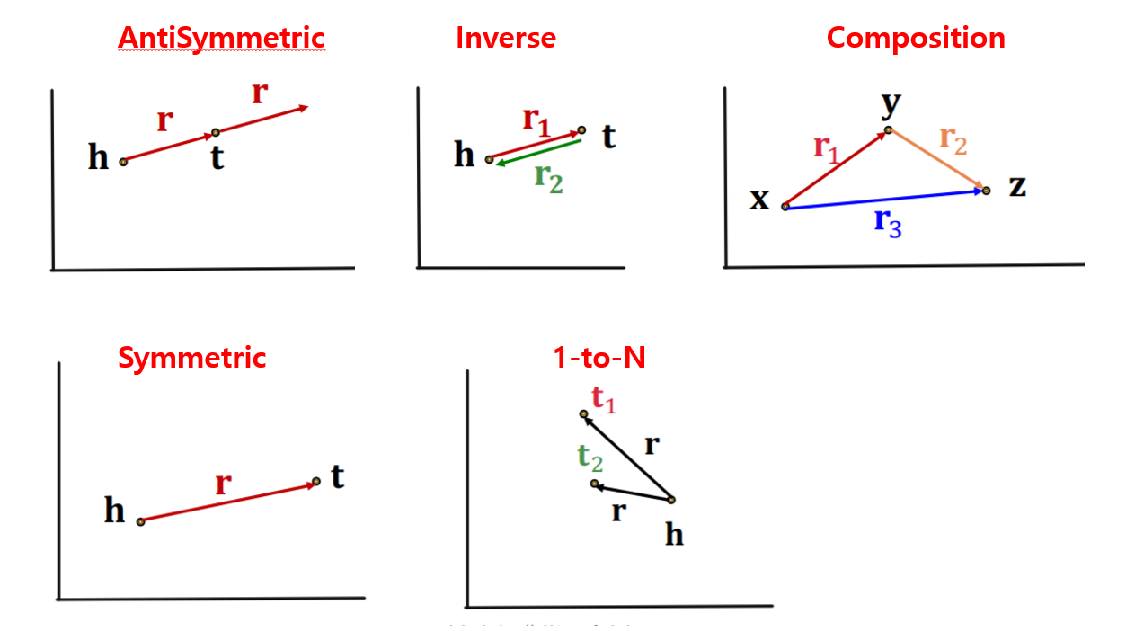
(2) Connectivity Patterns in KG
-
Symmetric :
- notation : \(r(h, t) \Rightarrow r(t, h)(r(h, t) \Rightarrow \neg r(t, h)) \quad \forall h, t\)
- example : roommate
- Inverse :
- notation : \(r_{2}(h, t) \Rightarrow r_{1}(t, h)\).
- example : (advisor, advisee)
- Composition (Transitive)
- notation : \(r_{1}(x, y) \wedge r_{2}(y, z) \Rightarrow r_{3}(x, z) \quad \forall x, y, z\).
- example : (mother’s husband = father)
- 1-to-N
- notation : \(r\left(h, t_{1}\right), r\left(h, t_{2}\right), \ldots, r\left(h, t_{n}\right) \text { are all True. }\)
- example : r = StudentsOf
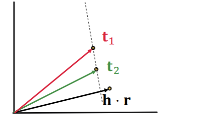
(3-1) TransE
- idea : \(\mathbf{h}+\mathbf{r} \approx \mathbf{t}\)
- scoring function : \(f_{r}(h, t)=- \mid \mid \mathbf{h}+\mathbf{r}-\mathbf{t} \mid \mid\)
- loss : max margin loss
Relation Types
-
Antisymmetric (O)
- \(h+r=t\), but \(t+r \neq h\)
-
Inverse (O)
- \(h + r_2 =t\), we can set \(r_1 = -r_2\)
-
Composition (O)
- \[r_3 = r_1 + r_2\]
-
Symmetric (X)
- only if \(r=0\), \(h=t\)
-
1-to-N (X)
-
\(t_1\) and \(t_2\) will map same vector
although they are different entities
-
contradictory!
- \[t_1 = h+r = t_2\]
- \[t_1 \neq t_2\]
-
(3-2) TransR
TransE :
- translation of any relation in the SAME embedding space
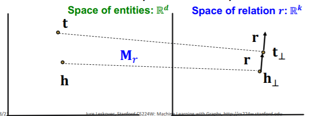
TransR :
- translation of relation in the DIFFERENT embedding space
- notation
- model “entities” as vectors in the entity space \(\mathbb{R}^{d}\)
- model “each relation” as vector in relation space \(\mathbf{r} \in \mathbb{R}^{k}\)
- with \(\mathbf{M}_{r} \in \mathbb{R}^{k \times d}\) as projection matrix
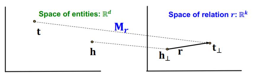
- \(\mathbf{h}_{\perp}=\mathbf{M}_{r} \mathbf{h}, \mathbf{t}_{\perp}=\mathbf{M}_{r} \mathbf{t}\).
- score function : \(f_{r}(h, t)=-\left \mid \mid \mathbf{h}_{\perp}+\mathbf{r}-\mathbf{t}_{\perp}\right \mid \mid\)
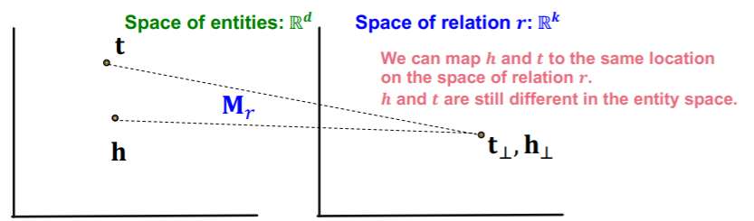
Relation Types
-
Symmetric (O)
- \(\mathbf{r}=0, \mathbf{h}_{\perp}=\mathbf{M}_{r} \mathbf{h}=\mathbf{M}_{r} \mathbf{t}=\mathbf{t}_{\perp}\).
-
Assymetric (O)
-
\(\mathbf{r} \neq 0, \mathbf{M}_{r} \mathbf{h}+\mathbf{r}=\mathbf{M}_{r} \mathbf{t}\).
then, \(\mathbf{M}_{r} \mathbf{t}+\mathbf{r} \neq \mathbf{M}_{r} \mathbf{h}\)
-
-
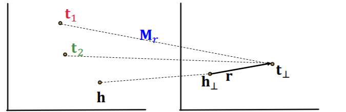
- 1-to-N (O)
- we can learn \(\mathbf{M}_{r}\) so that \(\mathbf{t}_{\perp}=\mathbf{M}_{r} \mathbf{t}_{1}=\mathbf{M}_{r} \mathbf{t}_{2}\)
-
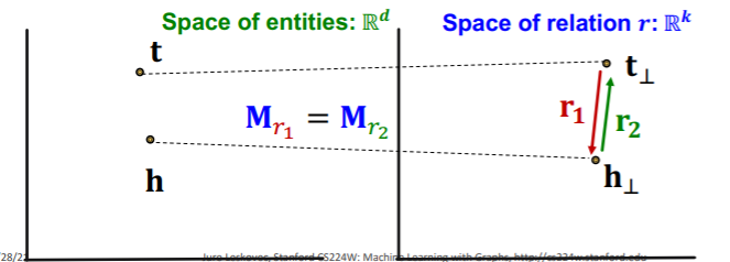
Inverse (O)
-
\[\mathbf{r}_{2} =-\mathbf{r}_{1}, \mathbf{M}_{r_{1}}=\mathbf{M}_{r_{2}}\]
then, \(\mathbf{M}_{r_{1}} \mathbf{t}+\mathbf{r}_{1} =\mathbf{M}_{r_{1}} \mathbf{h} \text { and } \mathbf{M}_{r_{2}} \mathbf{h}+\mathbf{r}_{2}=\mathbf{M}_{r_{2}} \mathbf{t}\)
-
\[\mathbf{r}_{2} =-\mathbf{r}_{1}, \mathbf{M}_{r_{1}}=\mathbf{M}_{r_{2}}\]
- Composition (O)
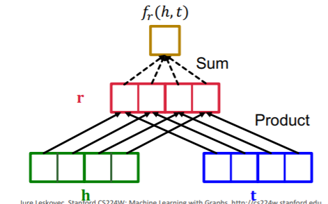
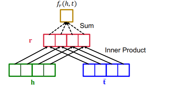
(3-3) DistMult
-
adopt BILINEAR modeling!
-
score function : \(f_{r}(h, t)=<\mathbf{h}, \mathbf{r}, \mathbf{t}>=\sum_{i} \mathbf{h}_{i} \cdot \mathbf{r}_{i} \cdot \mathbf{t}_{i}\).
- can be seen as cosine similarity, between \(h\cdot r\) & \(t\)
Relation Types
- 1-to-N (O)
- \(\left\langle\mathbf{h , r}, \mathbf{t}_{1}\right\rangle=\left\langle\mathbf{h}, \mathbf{r}, \mathbf{t}_{2}\right\rangle\).
- Symmetric (O)
- \(f_{r}(h, t)=<\mathbf{h}, \mathbf{r}, \mathbf{t}>=\sum_{i} \mathbf{h}_{i} \cdot \mathbf{r}_{i} \cdot \mathbf{t}_{i}=<\mathbf{t}, \mathbf{r}, \mathbf{h}>=f_{r}(t, h)\).
-
AntiSymmetric (X)
-
\(f_{r}(h, t)=<\mathbf{h}, \mathbf{r}, \mathbf{t}>=<\mathbf{t}, \mathbf{r}, \mathbf{h}>=f_{r}(t, h)\).
( \(r(h,t)\) & \(r(t,h)\) will always have same score )
-
-
Inverse (X)
-
\(f_{r_{2}}(h, t)=\left\langle\mathbf{h}, \mathbf{r}_{2}, \mathbf{t}\right\rangle=\left\langle\mathbf{t}, \mathbf{r}_{1}, \mathbf{h}\right\rangle=f_{r_{1}}(t, h)\).
( this means \(\mathbf{r}_{2}=\mathbf{r}_{1}\) )
-
-
Composition (X)
-
union of the hyperplane induced by multi-hops of relations
can not be expressed using a single hyperplane!
-
(3-4) ComplEx
- based on DistMult
- embeds entities&relations in COMPLEX vector space
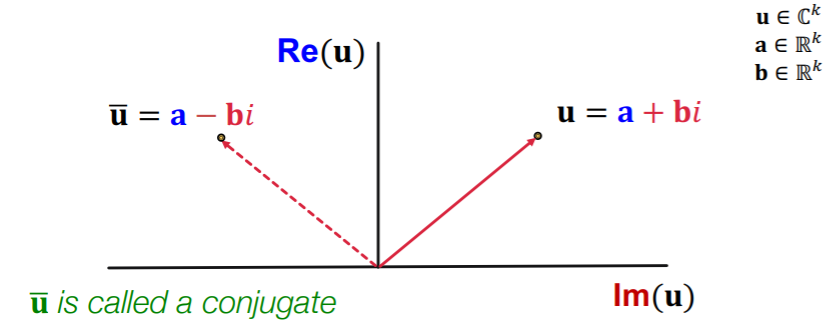
- Score function : \(f_{r}(h, t)=\operatorname{Re}\left(\sum_{i} \mathbf{h}_{i} \cdot \mathbf{r}_{i} \cdot \overline{\mathbf{t}}_{i}\right)\).
Relation Types
- Antisymmetric (O)
- High \(f_{r}(h, t)=\operatorname{Re}\left(\sum_{i} \mathbf{h}_{i} \cdot \mathbf{r}_{i} \cdot \overline{\mathbf{t}}_{i}\right)\).
- Low \(f_{r}(t, r)=\operatorname{Re}\left(\sum_{i} \boldsymbol{t}_{i} \cdot \mathbf{r}_{i} \cdot \overline{\boldsymbol{h}}_{i}\right)\)
- Symmetric (O)
- when \(Im(r)=0\)….
- \(\begin{aligned} f_{r}(h, t)&=\operatorname{Re}\left(\sum_{i} \mathbf{h}_{i} \cdot \mathbf{r}_{i} \cdot \overline{\mathbf{t}}_{i}\right)=\sum_{i} \operatorname{Re}\left(\mathbf{r}_{i} \cdot \mathbf{h}_{i} \cdot \overline{\mathbf{t}}_{i}\right) \\ &=\sum_{i} \mathbf{r}_{i} \cdot \operatorname{Re}\left(\mathbf{h}_{i} \cdot \overline{\mathbf{t}}_{i}\right)=\sum_{i} \mathbf{r}_{i} \cdot \operatorname{Re}\left(\overline{\mathbf{h}}_{i} \cdot \mathbf{t}_{i}\right)\\&=\sum_{i} \operatorname{Re}\left(\mathbf{r}_{i} \cdot \overline{\mathbf{h}}_{i} \cdot \mathbf{t}_{i}\right)=f_{r}(t, h) \end{aligned}\).
- Inverse (O)
- \(\mathbf{r}_{1}=\overline{\mathbf{r}}_{2}\).
- Complex conjugate of \(\mathbf{r}_{2}=\underset{\mathbf{r}}{\operatorname{argmax}} \operatorname{Re}(<\mathbf{h}, \mathbf{r}, \overline{\mathbf{t}}>)\) is exactly \(\mathbf{r}_{1}=\underset{\mathbf{r}}{\operatorname{argmax}} \operatorname{Re}(<\mathbf{t}, \mathbf{r}, \overline{\mathbf{h}}>)\).
- Composition (X)
- 1-to-N (O)
(3-5) Summary