KAN: Kolmogorov–Arnold Networks (arxiv 2024)
Liu, Ziming, et al. "Kan: Kolmogorov-arnold networks." arXiv preprint arXiv:2404.19756 (2024)
( https://arxiv.org/pdf/2404.19756 )
Contents
- Abstract
- MLP vs. KAN
- KAT
- Limitation of KAT
- How to solve?
- KAN Architecture
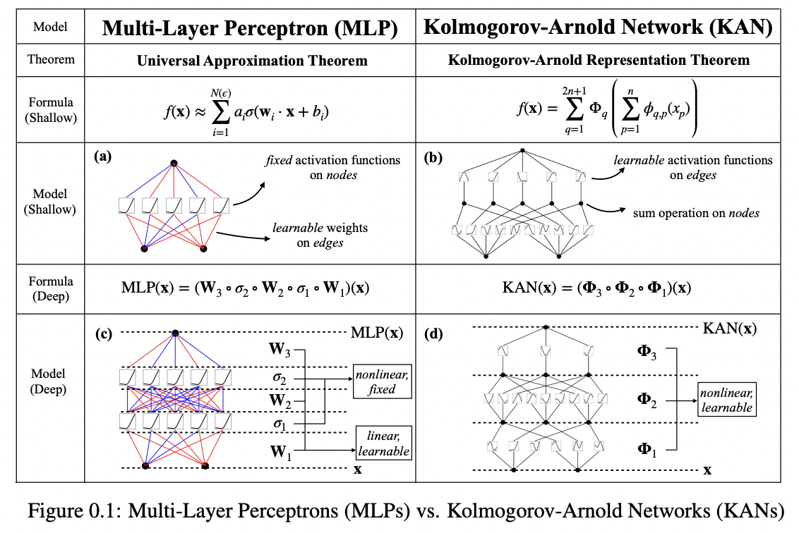
- MLP vs. KAN
- Acitvation fuction
- B-spline
- Interpretability
- Sparsification
- Visualization
- Pruning
1. Abstract
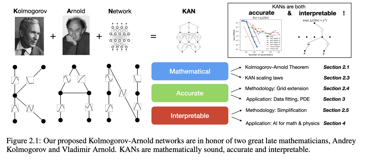
- (1) Based on KAT (Kolmogorov-Arnold representation theorem)
- (2) Promising alternatives to MLPs
- (3) MLP vs. KAN
- MLP: Fixed activation functions, on nodes (“neurons”)
- KAN: Learnable activation functions, on edges (“weights”)
- KANs have no linear weights at all
- Every weight parameter is replaced by a univariate function parametrized as a spline
- (4) Excel at both accuracy and interpretability
2. MLP vs. KAN


3. KAT
Kolmogorov-Arnold Representation theorem
\(f(\mathbf{x})=f\left(x_1, \cdots, x_n\right)=\sum_{q=1}^{2 n+1} \Phi_q\left(\sum_{p=1}^n \phi_{q, p}\left(x_p\right)\right)\).
\(\rightarrow\) Every other function can be written using univariate functions and sum.
(1) Limitation of KAT
“Learning a high-dimensional function” boils down to “Learning a polynomial number of 1D functions”??
\(\rightarrow\) However, these 1D functions can be non-smooth and even fractal, so they may not be learnable in practice [19, 20].
\(\rightarrow\) Regarded as theoretically sound but practically useless… :(
(2) How to solve?
KAN = optimistic about the usefulness of the KAT for ML!
How?
-
(1) Need not stick to the original Eq. (2.1) which has only two-layer nonlinearities and a small number of terms (2n + 1) in the hidden layer
\(\rightarrow\) Generalize the network to arbitrary widths and depths
-
(2) Most functions in science and daily life are often smooth and have sparse compositional structures, potentially facilitating smooth Kolmogorov-Arnold representations
4. KAN Architecture
(1) MLP vs. KAN
- (MLP) \(\operatorname{MLP}(\mathbf{x})=\left(\mathbf{W}_3 \cdot \sigma_2 \cdot \mathbf{W}_2 \cdot \sigma_1 \cdot \mathbf{W}_1\right)(\mathbf{x})\)
- (KAN) \(\operatorname{KAN}(\mathbf{x})=\left(\Phi_3 * \Phi_2 * \Phi_1\right)(\mathbf{x})\).
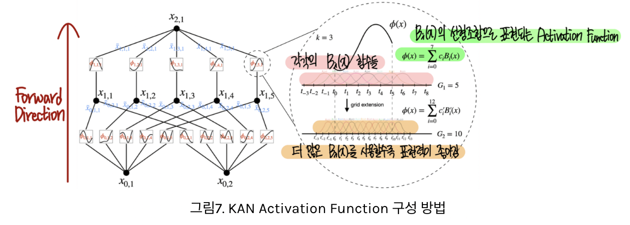
(2) Activation function
Activation fuction: \(\phi(x)=w(b(x)+\operatorname{spline}(x))\)
- (1) Basis function: \(b(x)=\operatorname{silu}(x)=x /\left(1+e^{-x}\right)\)
- (2) Spline: \(\operatorname{spline}(x)=\sum_i c_i B_i(x)\).
- Linear combination of B-spline

( https://ffighting.net/deep-learning-paper-review/vision-model/kan/ )
(3) B-spline (Basis spline)
\(\rightarrow\) Combining multiple basis functions to create smooth and flexible curves
(1) Definition: Piecewise-defined polynomial curve constructed as a linear combination of basis functions
-
Each basis function: has a local influence
( = changes to control points or parameters only affect the corresponding part of the curve )
(2) Characteristics
- a) Piecewise Polynomial Representation
- B-spline = Consists of “several” polynomial segments joined together.
- The degree of the polynomials determines the degree of the B-spline.
- b) Smoothness
- Continuity at the segment boundaries depends on the spline’s degree and the configuration of the knot vector
-
c) Knot Vector
-
Divides the parameter domain into intervals
& Determines where and how the polynomial pieces connect.
-
Uniform (equally spaced knots) vs. non-uniform (unequally spaced knots)
-
- d) Local Control
- Modifying a control point affects only the curve’s local segment, thanks to the localized influence of the basis functions.
5. Interpretability
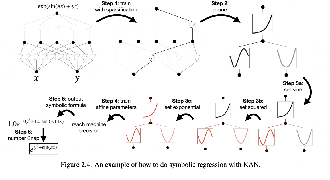
Start from a large enough KAN and train it with “sparsity regularization” followed by “pruning”
\(\rightarrow\) These pruned KANs are much more interpretable than non-pruned ones
To make KANs maximally interpretable, requires below simplification techniques !

(1) Sparsification
(MLP) \(L_1\) regularization of linear weights
(KAN) Requires two modifications
-
(1) There is no linear “weight” in KANs
\(\rightarrow\) Linear weights are replaced by learnable activation functions, so we should define the L1 norm of these activation functions.
-
(2) Find \(L_1\) to be insufficient for sparsification of KANs
\(\rightarrow\) Additional entropy regularization is necessary
a) \(L_1\) norm of ..
- (1) Activation function \(\phi\) : Average magnitude over its \(N_p\) inputs
- \(\mid \phi \mid _1 \equiv \frac{1}{N_p} \sum_{s=1}^{N_p} \mid \phi\left(x^{(s)}\right) \mid\).
- (2) KAN layer \(\boldsymbol{\Phi}\) (with \(n_{\text {in }}\) inputs and \(n_{\text {out }}\) outputs)
- \(L_1\) norm of \(\boldsymbol{\Phi}\) = Sum of L1 norms of all activation functions
- \(\mid \Phi \mid _1 \equiv \sum_{i=1}^{n_{\text {ien }}} \sum_{j=1}^{n_{\text {out }}} \mid \phi_{i, j} \mid _1\).
b) Entropy of \(\Phi\):
- \(S(\Phi) \equiv-\sum_{i=1}^{n_{\text {in }}} \sum_{j=1}^{n_{\text {out }}} \frac{ \mid \phi_{i, j} \mid _1}{ \mid \Phi \mid _1} \log \left(\frac{ \mid \phi_{i, j} \mid _1}{ \mid \Phi \mid _1}\right)\).
c) Total Loss:
\(\ell_{\text {total }}=\ell_{\text {pred }}+\lambda\left(\mu_1 \sum_{l=0}^{L-1} \mid \boldsymbol{\Phi}_l \mid _1+\mu_2 \sum_{l=0}^{L-1} S\left(\boldsymbol{\Phi}_l\right)\right)\).
-
\(\mu_1, \mu_2\) : Relative magnitudes
( usually set to \(\mu_1=\mu_2=1\) )
-
\(\lambda\): controls overall regularization magnitude
(2) Visualization
To get a sense of magnitudes, we set the transparency of an activation function \(\phi_{l, i, j}\) proportional to \(\tanh \left(\beta A_{l, i, j}\right)\) where \(\beta=3\).
\(\rightarrow\) Functions with small magnitude appear faded out ( allow us to focus on important ones )
(3) Pruning
May also want to prune the network to a smaller subnetwork
Sparsify KANs on the node level (rather than on the edge level).
For each node (say the \(i^{\text {th }}\) neuron in the \(l^{\text {th }}\) layer),
- Incoming score: \(I_{l, i}=\max _k\left( \mid \phi_{l-1, i, k} \mid _1\right)\).
- Outcoming score: \(O_{l, i}=\max _j\left( \mid \phi_{l+1, j, i} \mid _1\right)\)
\(\rightarrow\) Important if both incoming and outgoing scores are greater than a threshold hyperparameter \(\theta=10^{-2}\) by default.
