All about Mistral

All about “Mistral”

(Reference: https://www.youtube.com/watch?v=UiX8K-xBUpE)

Contents

1. Introduction to Mistral
   1. Transformer vs. Mistral
   2. Mistral vs. LLaMA
2. Mistral vs. Mixtral
3. Sliding Window Attention (SWA)
   1. w/o SWA vs. w/SWA
   2. Details
4. KV-Cache
   1. KV-Cache
   2. Rolling Buffer Cache
   3. Pre-fill & Chunking
5. Sparse MoE
6. Model Sharding
7. Optimizing inference with multiple prompts

1. Introduction to Mistral

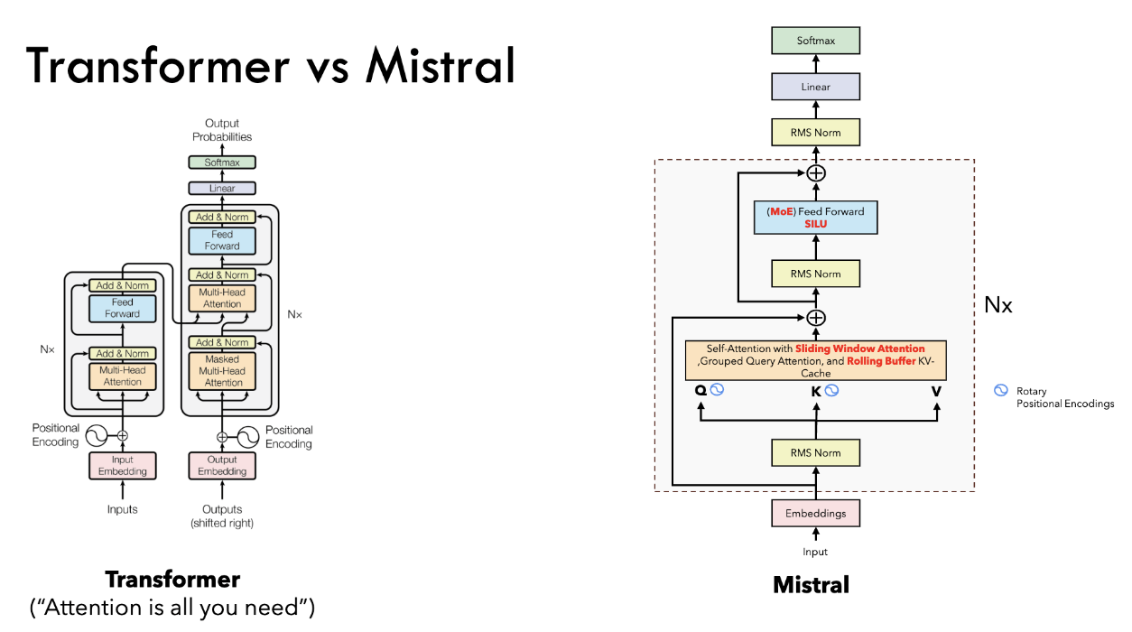
(1) Transformer vs. Mistral

• (naive) Transformer = Encoder + Decoder
• Mistral = Decoder-only model (like LLaMA)

(2) Mistral vs. LLaMA

• (1) Attention \(\rightarrow\) Sliding window attention
• (2) Rolling Buffer
• (3) FFN \(\rightarrow\) MoE (for Mixtral)
• Both methods uses
  • (1) GQA (Grouped query attention)
  • (2) RoPE (Rotary Positional Embedding)

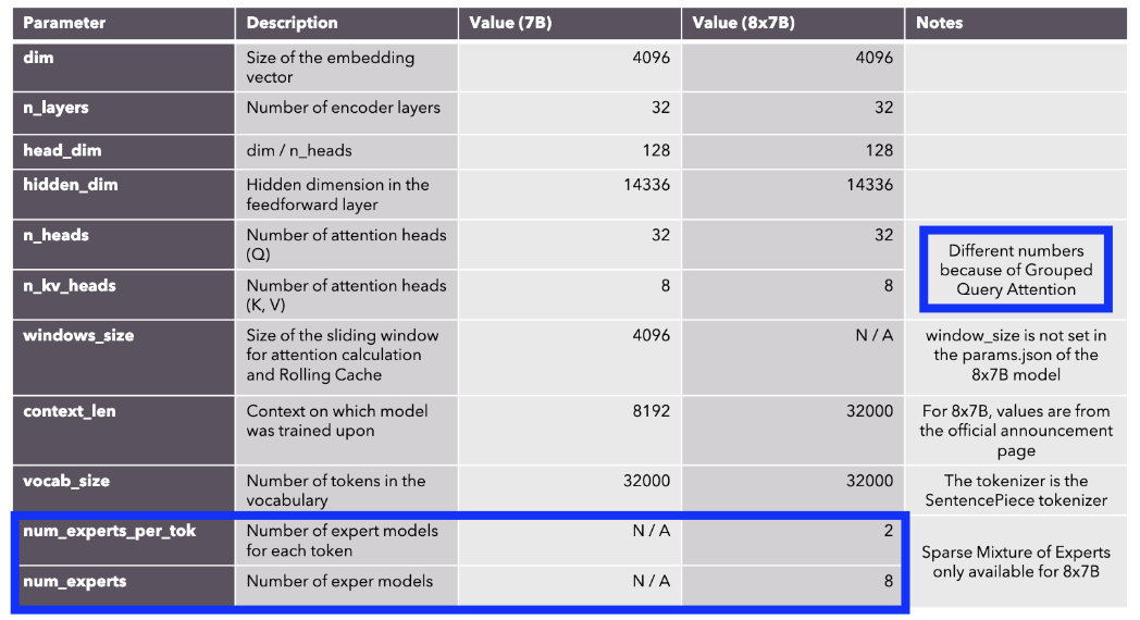
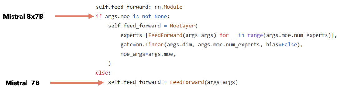
2. Mistral vs. Mixtral

Depends on the usage of MoE!

• Mistral: MoE (X) … 7B
• Mixtral: MoE (O) … 8 experts of 7B

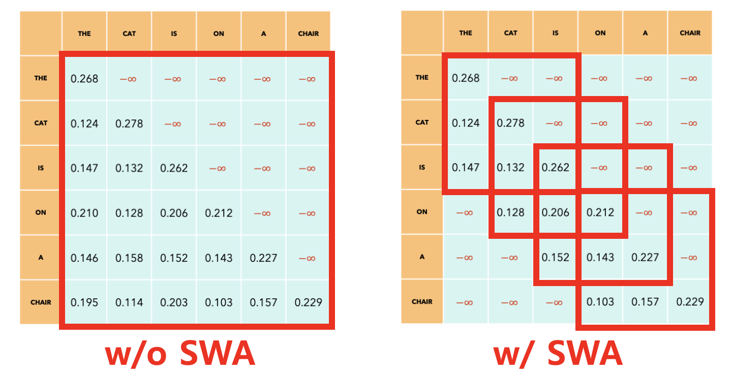
3. Sliding Window Attention (SWA)

(1) w/o SWA vs. w/ SWA

( sliding window size = 3 )

(2) Details

1. [Efficiency] Reduce the # of dot products

2. [Trade-off] May lead to degradation, as less interaction btw tokens

   \(\rightarrow\) But still, much more efficient!

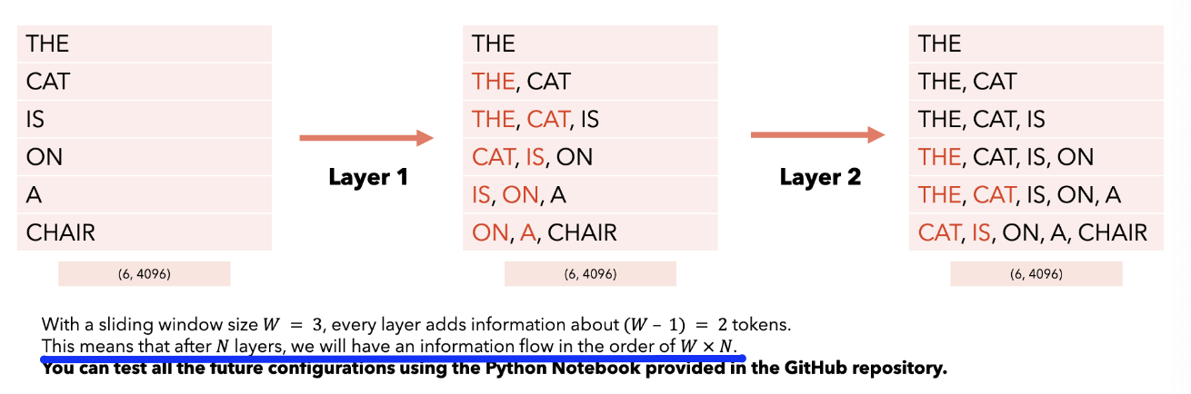
3. [Receptive field] Can still allow one token to watch outside the window (due to multiple layers)

4. KV-Cache

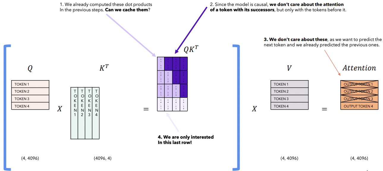
(1) KV-Cache

Goal: Faster inference!

At each step of the inference, only interested in the last token!

• As ONLY the last token is projected to linear layer (to predict the next token)

Nonetheless, model needs all the previous tokens to constitute its context

\(\rightarrow\) Solution: KV Cache

a) Inference w/o KV Cache

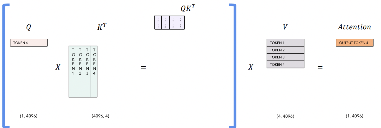
b) Inference w/ KV Cache

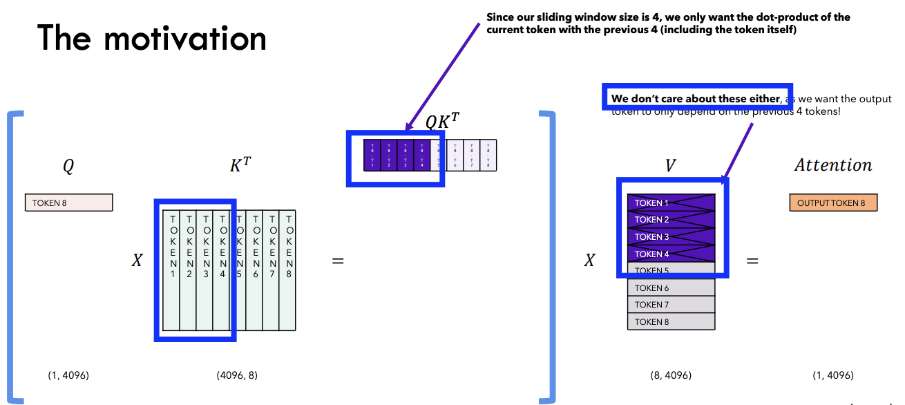
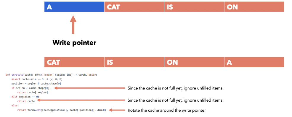
(2) Rolling Buffer Cache

“KV-Cache” + “Sliding window attention”

\(\rightarrow\) No need to keep ALL the previous tokens in the cache!

( only limit to the “latest \(W\) tokens”)

Example:

• Sentence: “The cat is on a chair”
• Window size (\(W\)) = 4
• Current token: \(t=4\) (chair)

\(t=3\) : [The, cat, is, on]

should become

\(t=4\) : [cat, is, on, a]

\(\rightarrow\) By “unrolling” ( or unrotating )

(3) Pre-fill & Chunking

a) Inference with LLM

Infernce with LLM

• Use a prompt & Generate tokens “ONE BY ONE” (using the previous tokens)

Inference with LLM + “KV-Cache”

• Add all the prompt tokens to the KV-Cache

b) Motivation

[Motivation] We know all the prompts in advance! ( = no need to generate )

\(\rightarrow\) Why not “PREFILL” the KV-Cache using the “tokens of the PROMPT”?

( + What if the prompt is toooo long? )

Solution:

• (1) Prefilling: prefill the kv-cache using the tokens of the prompt
• (2) Chunking: divide the prompt into chunkks (of size \(W\) = window size)

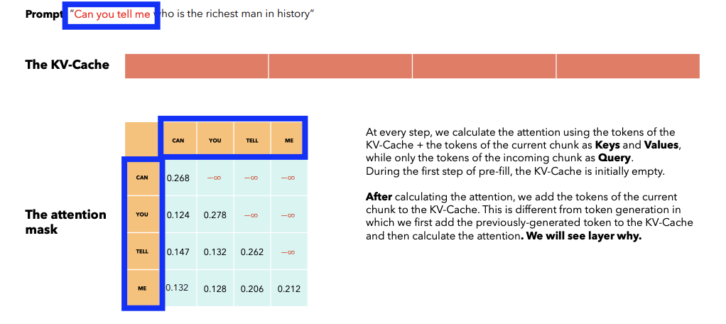
c) Example

Setting:

• Large (Long) prompt + \(W=4\)

• Sentence = “Can you tell me who is the richest man in history?”

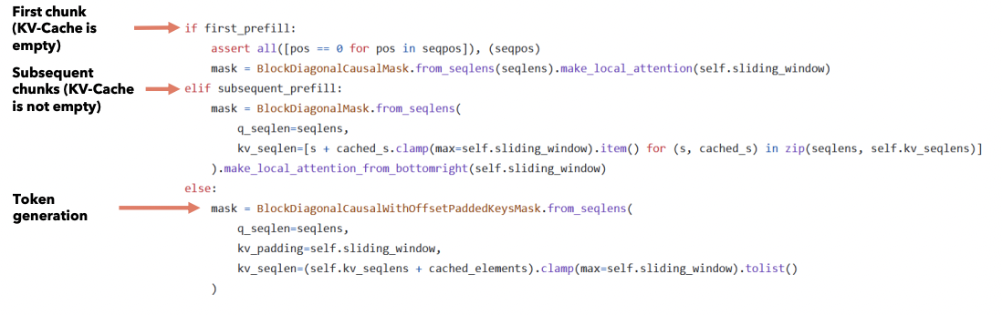
Step 1) First prefill

• Fill the first \(W\) tokens in the KV-Cache

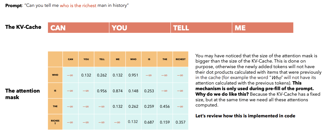
Step 2) Subsequent prefill

• Fill the next \(W\) tokens in the KV-Cache

• Attention masked is calculated using ….

  • (1) KV-Cache (Can, you, tell, me)
  • (2) Current chunk (who is the richest)

  \(\rightarrow\) \(\therefore\) Size of attention mask can be bigger than \(W\)

Step 3) Generation

• Size of attention mask = \(W\)

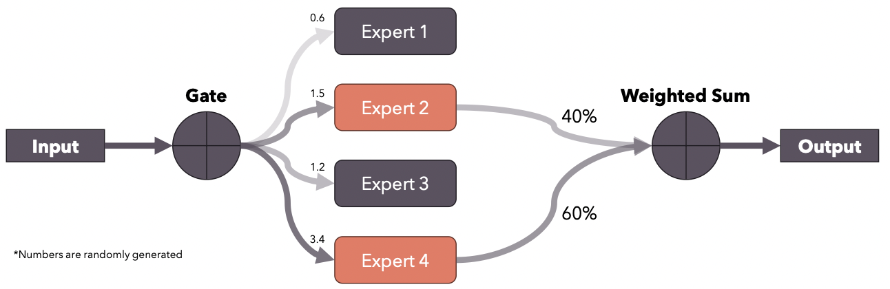
5. Sparse MoE

Mixture of Experts: Ensemble technique

• Multiple “expert” models
  • Each trained on a subset of the data
  • Each model specializes on it
• Output of the experts are combined

Mistral 8x7B: Sparse Mixture of Experts (SMoE)

• Only 2 out of 8 experts are used for every token
• Gate: Produces logits \(\rightarrow\) Used to select the top-k experts

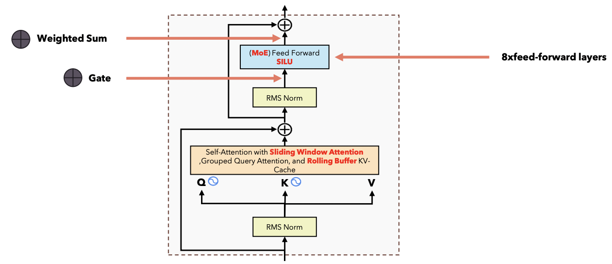
Details

• Experts = FFN layers
• Architectures: Each Encoder layer is comprised of …
  • (1) Single Self-Attention mechanism
  • (2) Mixture of experts of 8 FFN
    • Gate function selects the top 2 experts

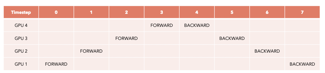
6. Model Sharding

Example) Pipeline parallelism (PP)

• Mistral = 32 Encoder layers
  • 4 GPUs x 8 layers

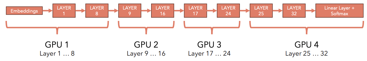
\(\rightarrow\) Not very efficient! Only one GPU is working at a time! How to solve?

Before

After

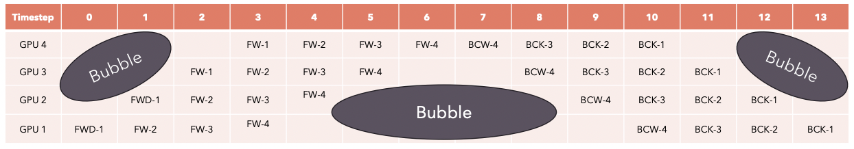
• Divide batch into smaller microbatches!
• Gradient accumulation: Gradients for each microbatch is accumulated!

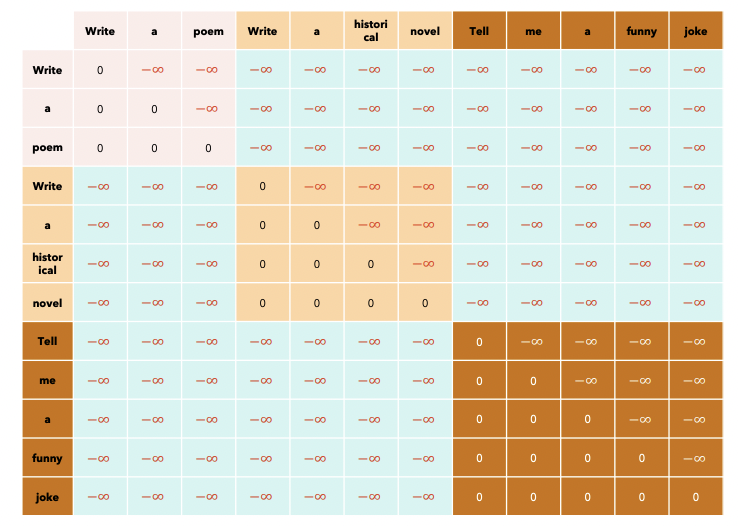
7.Optimizing inference with multiple prompts

(1) Problem

Example) Prompt of 3 different users

• Prompt 1: “Write a poem” (3 tokens)
• Prompt 2: “Write a historical novel” (4 tokens)
• Prompt 3: “Tell me a funny joke” (5 tokens)

( Note that we cannot use )

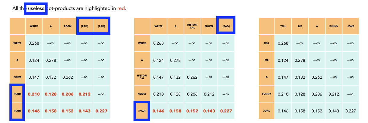
(2) Solution

Into a SINGLE sequence!

( + Keep track of the “length of each prompt” when we calculate the output )

\(\rightarrow\) by using xformers BlockDiagonalCausalMask