Byte Latent Transformer; Patches Scale Better Than Tokens

Byte Latent Transformer: Patches Scale Better Than Tokens

Pagnoni, Artidoro, et al. "Byte Latent Transformer: Patches Scale Better Than Tokens." arXiv preprint arXiv:2412.09871 (2024).

참고:

• https://aipapersacademy.com/byte-latent-transformer/
• https://arxiv.org/pdf/2412.09871

Contents

1. Introduction
2. Recap: Byte into patches
   1. 4-Strided Approach
   2. Byte-Pair Encoding (BPE)
   3. Space Patching
   4. Entropy-based Patching
3. BLT Architecture
   1. Local Encoder
   2. Latent Transformer
   3. Local Decoder
4. Local Encoder & Local Decoder
   1. Local Encoder
   2. Local Decoder

1. Introduction

LLM = “tokenizer” before the Transformer

• Role: Converts text into tokens

  ( = which are part of the vocabulary of the LLM )

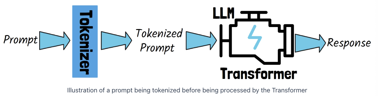
Tokens are provided by an external component

\(\rightarrow\) The model cannot decide whether to allocate more compute to a certain token

( =All tokens are treated the same )

Problems?

• Some tokens are much harder to predict than others.

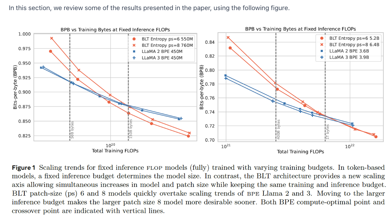
Byte Latent Transformer (BLT)

“Byte Latent Transformer: Patches Scale Better Than Tokens.”

Byte Latent Transformer (BLT)

• Tokenizer-free architecture = Learns from raw byte data

• Processing the sequence byte by byte results in very large sequences

  \(\rightarrow\) Scaling issues ..? How to solve?

• Solution: Dynamically groups bytes into patches

  ( & Performs most of its processing on these patches )

2. Recap: Byte into patches

Previous works) How to divide the Byte Sequence into Patches?

• Ex) “Daenerys Targaryen is in Game of Thrones, a fantasy epic by George R.R. Martin.”

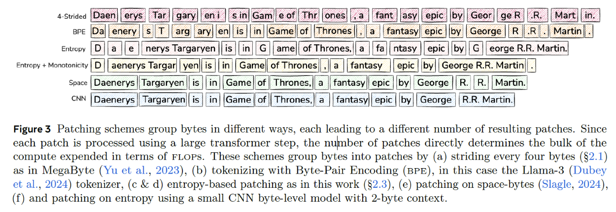
(a) 4-Strided Approach

Patch = Fixed size of 4 bytes

• Pros) Simplicity
• Cons)
  • (1) Does not dynamically allocate compute where it is needed the most
  • (2) Similar byte sequences may suffer from inconsistent patching

(b) Byte-Pair Encoding (BPE)

Patch = Subword tokenization

• Used in many LLMs (e.g., LLaMA 3)

(c) Space Patching

Patch = by space

• Start a new patch after any space-like byte
• Pros)
  • (1) Consistent patching
  • (2) Compute is allocated for every word
• Cons)
  • (1) Does not fit all languages and domains, such as math.
  • (2) Cannot vary patch size, as it is determined by the word’s length.

(d) Entropy-based Patching

Dynamic allocation of compute where it is needed the most

• Entropy = uncertainty
• Entropy is calculated over the prediction of the next byte
  • Via a small byte-level language model trained for this purpose.

\(\rightarrow\) High uncertainty for predicting the next token = Good hint that the next byte is a hard one to predict

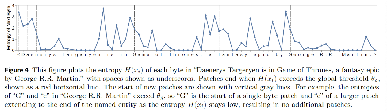
Entropy vs. Entropy + Monotonicity

Entropy: \(H\left(x_t\right)>\theta_g\)

• Setting a threshold for the entropy for predicting the next byte

Entropy + Monotnoicity: \(H\left(x_t\right)-H\left(x_{t-1}\right)>\theta_r\)

• Not the entropy value, but rather the difference between the entropy of predicting the next byte and the entropy for predicting the current byte

3. BLT Architecture

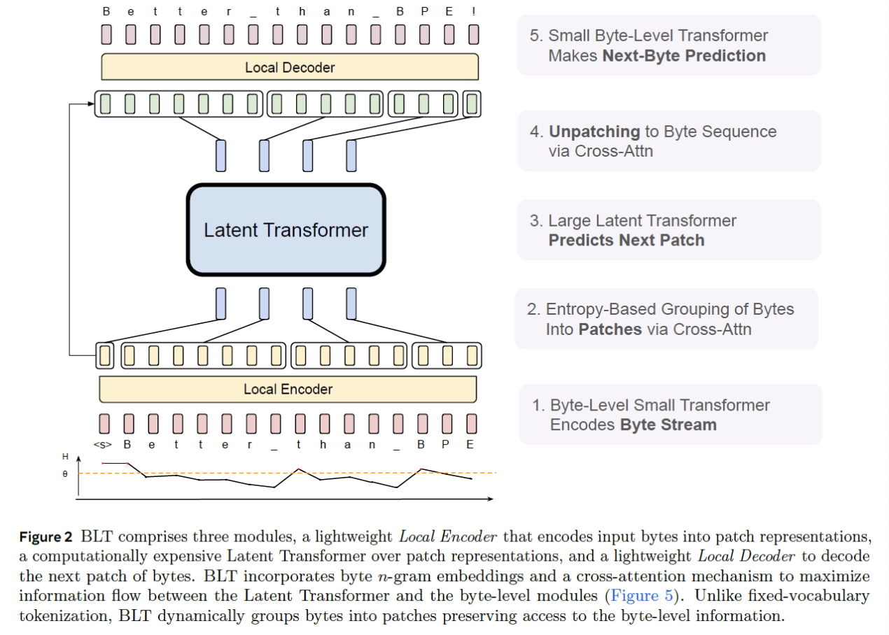
Three key modules

• (1) Local Encoder
• (2) Latent Transformer
• (3) Local Decoder

(1) Local Encoder

1-1) Input: Byte embedding

• Combination of multiple n-gram embeddings

  ( to provide context about the preceding bytes )

  • \(f(\text{byte1})\) (X)
  • \(f(\text{byte1,2,..,n})\) (O)

1-2) Local Encoder

• Encodes the input byte embeddings

  (via Lightweight byte-level Transformer)

• Responsible for creating the patch sequence

  • (1) Patchify: based on the entropy method (Next Byte Prediction)
  • (2) Patch embedding: Cross-attention btw
    • (1) Byte sequence
    • (2) Initial patch sequence.

(2) Latent Transformer

2-1) Input: Patch sequence

2-2) Transformer: Main component of BLT

• Processes the patches & provide output patch representations

(3) Local Decoder

3-1) Input: Patch sequence

3-2) Decoder:

• Unpatches the patch sequence \(\rightarrow\) To a byte sequence

• How? via cross-attention with the output of the Local Encoder,

• Architecture: Small byte-level Transformer

  ( used to predict the next byte )

4. Local Encoder & Local Decoder

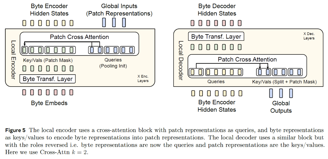
(1) Local Encoder

Inputs)

• (1) Byte Embeddings \(\rightarrow\) pass through Transformer (masked self-attention)
• (2) Initial patch sequence representations = by pooling (\(k=2\))
  • Each patch gets two vectors for its representation

• Patch Cross Attention

  • Q,K,V

    • (K,V) = with (1)
    • (Q) = with (2)

  • Masking (to attend only preceding bytes)

    • Byte embeddings can have context from previous patches

      ( \(\because\) n-gram embeddings & masked byte-level Transformer layer)

Output) Encoded bytes & Patch representation’s hidden states

(2) Local Decoder

Input)

• (1) Encoded bytes (from the Local Encoder)
• (2) Patch outputs (from the Latent Transformer)

Decoding = Inversion of the Local Encode.