Causal Inference Meets Deep Learning: A Comprehensive Survey

Abstract
Introduction
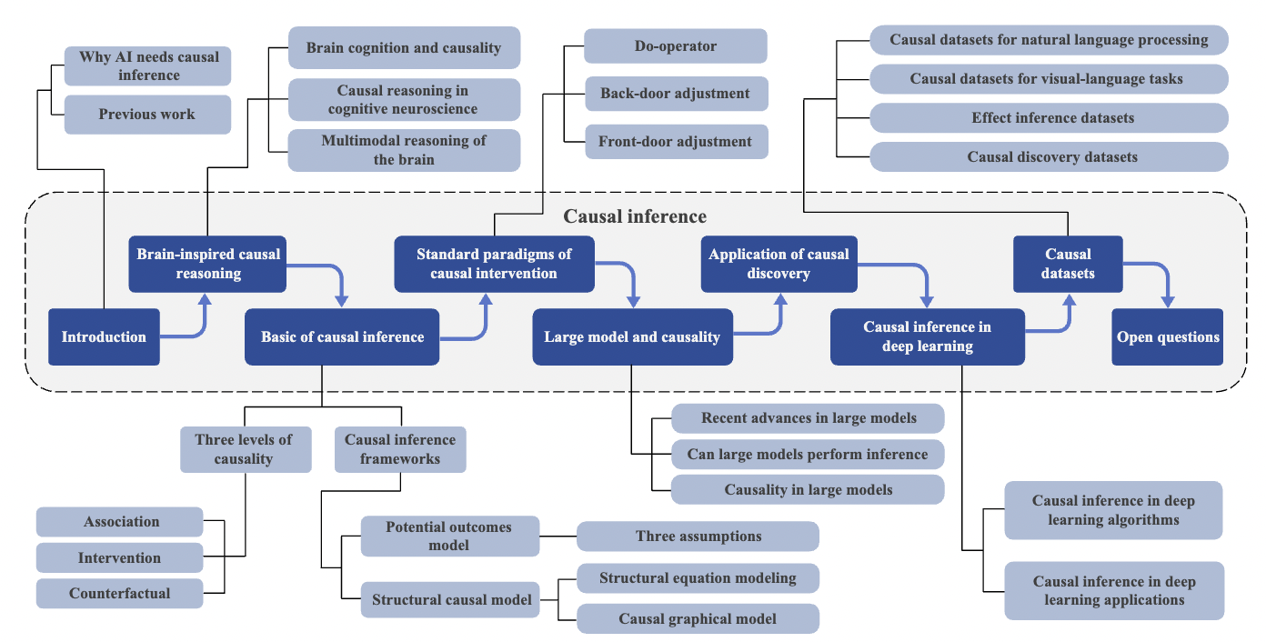
1. Overview and organization
2. Why AI needs causal inference
  1. Improved accuracy of decision-making
  2. Improving model generalization & robustness
  3. Improving the interpretability of models
3. Previous works
Brain-Inspired Reasoning
Basic of Causal Inference
1. Three levels of causality
  1. Association
  2. Intervention
  3. Counterfactuals
2. The basic paradigim of causal intervention
  1. Potential outcomes model (POM)
  2. Structural causal modeling (SCM)
  3. Summary of POM vs. SCM

Abstract

(1) DL models = May learn “spurious correlations”

\(\rightarrow\) Reduce robustness & interpretability
(2) Causal inference

\(\rightarrow\) Offers more “stable and interpretable” alternatives

Goal of this paper

= (2) Causal learning concepts + Integration with (1) DL

1. Introduction

a) Limitation of DL

Overfitting to spurious correlations

\(\rightarrow\) Limiting generalization and robustness
Self-/semi-supervised and reinforcement learning

\(\rightarrow\) Focus heavily on data quantity

b) Causal Learning

Proposed to enhance interpretability & trustworthiness
Growing interest!

\(\rightarrow\) To address “non-IID challenges” in complex settings
- e.g., Healthcare and autonomous driving

(1) Overview and organization

Goal of Causal Learning

Identify and reduce data bias & spurious correlations
New lens to understand DL model behavior and limitations
Improves model robustness

Splits into “two main areas”

(1) Causal “discovery”
“Identifies” causal structures from observed data
Data- and compute-intensive, making it less practical in DL
(2) Causal “inference”
- “Quantifies” the strength of known causal effects
- More applicable to DL tasks

DL often …

a) Assumes that “causal structure exists”
b) Focuses on “estimating causal effects” from observational data

\(\rightarrow\) This paper focuses on CAUSAL INFERENCE aspect within DL contexts

This paper

(1) Introduces core concepts of causal inference
(2) Reviews theoretical foundations and general frameworks for causal inference
(3) Summarizes how causal inference integrates with classical DL algorithms
(4) Describes cross-domain applications of causal inference in DL tasks
(5) Highlights common datasets & future research challenges in causal learning

(2) Why AI needs causal inference

a) Improved “accuracy” of decision-making
b) Improving “model generalization & robustness”
c) Improving the “interpretability” of models

a) Improved accuracy of decision-making

DL models

Lack interpretability
Struggle in safety-critical domains

Causal inference

Enables understanding of “cause-effect” relationships
Helps identify which variables truly influence outcomes
Enhances decision-making accuracy & robustness in AI systems

b) Improving model generalization & robustness

DL models

Suffer from weak generalization and robustness

(\(\because\) Reliance on data correlations)
Limitation in real-world shifts

Causal inference

Enables models to identify stable, interpretable relationships & adapt to distribution changes
Causal attention and latent variable approaches

\(\rightarrow\) Help distinguish genuine causes from spurious correlations

c) Improving the interpretability of models

Traditional interpretable ML methods

E.g., rule-based and local surrogate models

Causal learning

Contributes by constructing causal graphs for clearer explanation of model decisions
Interventions and counterfactuals help assess variable impact on predictions

Recent methods

Use causal inference to reveal model mechanisms
Design interpretable neural architectures

(3) Previous works

Pearl’s foundational survey

Key mathematical tools in causal inference
- Potential outcomes
- Counterfactuals
- Direct/indirect effects

Guo et al. and Chen et al.

Explored causal inference and discovery
Across various data types and variable paradigms

Moraffah et al.

Applied causal inference to TS tasks
e.g., Effect estimation and causal structure learning

Liang et al.

Discussed challenges like convergence in applying causal analysis to AI

Yao et al.

Focused on potential outcome frameworks in statistical and ML methods

Schölkopf

Emphasized links between graphical causal inference and AI/ML

Proposed causal representation learning
To improve generalization and adaptation

(Especially in reinforcement learning contexts)

Most prior work:

Emphasizes causal discovery and statistical learning
Limited integration of causal learning in DL

Luo et al. and others

Explored model interpretability via structural causal models, DAGs, and Bayesian networks

Causal deep learning (CDL) frameworks

Covering dimensions like structure, parameters, and time
Zhou et al.
- Investigated causality in deep generative models and LLMs, focusing on data generation mechanisms
Kaddour et al.
- Proposed a taxonomy for CausalML
- e.g., Areas like causal fairness and causal RL, but lacked application depth in CV, NLP, and graphs
Liu et al.
- Reviewed causal methods for visual representation learning
- Lacked comprehensive coverage and task-level examples
Feder et al.
- Addressed causal inference in NLP
- But with limited DL scope across other domains

This paper

Explores causal inference from a brain-inspired perspective
Discusses how large models contribute to causal reasoning
Integration of causal inference + DL
Offers rich categorization and novel cross-domain insights
Summarizes related work in a detailed table with models, dates, tasks, and attributes
Provides a comprehensive list of causal datasets

2. Brain-Inspired Reasoning

a) Human brain reasoning

Surpasses AI in handling open-ended, complex, and dynamic scenarios

b) Traditional AI

Limited by its inability to model real-world complexity mathematically

a + b) Brain-inspired AI

Aims to replicate human cognitive flexibility and adaptability
Current AI
- Excels in computation
- Lacks human-like inference and generalization
Advancing AI toward brain-like reasoning is the key!!

3. Basic of Causal Inference

(1) Three levels of causality

Causality

“Directional” relationship where one event causes another

( = “Cause-effect link” )
The Book of Why presents the “ladder of causality”

\(\rightarrow\) Outlining three distinct levels of causal understanding

a) Association

(= First level of causality )

Based on observing “correlations” w/o establishing cause
- Correlation: temporal (X), undirectional
- Causailiy: temporal (O), directional
Confounders = Variables that distort the observed relationship (btw two variables)
- Needs to be “controlled” (O), “removed” (X)

Feat. ChatGPT
A variable is a confounder if it usually meets these conditions:
	1.	It is a cause of the treatment (e.g., temperature affects ice cream sales)
	2.	It is a cause of the outcome (e.g., temperature affects drowning accidents)
	3.	It opens a backdoor path between the treatment and the outcome

b) Intervention

( = Second causal level )

Involving active “manipulation of variables”
Aims to reduce confounding

\(\rightarrow\) Crucial to estimate true causal effects
Focuses on average causal effect “across groups, not individuals”
Key methods:
- (1) Randomized controlled trials (RCT)
- (2) Observational studies (using the do-operator)
  - Allows causal estimation from observational data w/o experiments

c) Counterfactuals

( = Highest causal level )

Address “what if” scenarios
- By reasoning about alternative outcomes
(Unlike interventions) Explore “hypothetical” situations
- Beyond observed or manipulated data
Require modeling of both the actual & counterfactual worlds for comparison

(2) The basic paradigim of causal intervention

Various causal inference frameworks!

Two most commonly utilized approaches

(1) POM
(2) SCM

a) Potential outcomes model (POM)

(Also called Rubin Causal Model)

Defines outcomes as either …
- (1) Factual (= observed)
- (2) Counterfactual (= unobserved)
Only “one” potential outcome is realized per individual!

\(\rightarrow\) Limiting direct causal observation

Individual Treatment Effect (ITE)

Quantifies causal impact for a specific intervention at the individual level
\(\tau_i=Y_i(1)-Y_i(0)\).
- \(Y(t)\) : “potential” outcome when the treatment \(T=t\)

Fundamental challenge?

= Inability to observe both \(Y_i(1)\) and \(Y_i(0)\)

\(\rightarrow\) Thus, “counterfactual” approach must be used!

Three assumptions of POM

Assumption 1: SUTVA
Assumption 2: Ignorability assumption
Assumption 3: Positivity assumption

[Assumption 1: SUTVA]

( Stable unit treatment value assumption )

= Each unit is independent

This assumption has 2 implications:
- (1) Unit independence
  - Potential outcomes of any unit are not affected by the interventions of other units.
  - e.g., If the effects of drug A are studied, the outcome of one patient taking drug A will not change depending on whether or not other patients are taking drug A.
- (2) Treatment consistency
  - There should be no different forms/versions of the intervention that each unit receives that could lead to different potential outcomes.
  - e.g., If different doses of drug A lead to different outcomes in the clinical trial, then different doses of drug A should be treated as different treatments.

[Assumption 2: Ignorability assumption]

( = Unconfoundedness assumption )

(“모든 confounder가 X에 포함되어 있다면, 처치 할당은 랜덤한 것처럼 취급할 수 있다.”)

\(W \perp(Y(0), Y(1)) \mid X\).

Given a background variable \(X\), the treatment assignment \(W\) is independent of the potential outcome \(Y\).
Two individuals with the same background should have the same potential outcome regardless of the treatment they actually receive.
e.g., if 2 patients have the same background variable \(X\), the distribution of their potential recovery outcomes (health status with and without treatment) should be the same regardless of whether they receive treatment or not.

[Assumption 3: Positivity assumption]

\(P(W=w \mid X=x)>0, \forall w \text { and } x\).

Allows every variable to be addressed by each intervention
e.g., Regardless of a patient’s variable \(X\), they will have a certain probability of receiving either drug \(A\) or drug \(B\).
i.e., There will not be a situation in which only drug \(A\) and not drug \(B\) is used for a certain class of people.
Ensures that all possible treatment outcomes can be observed to effectively estimate causal effects.

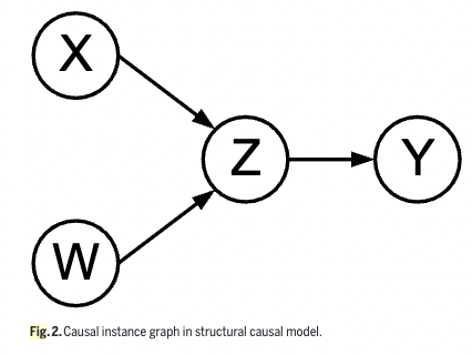
b) Structural causal modeling (SCM)

Uses “causal graphs” and “equations” to model causal relationships

Causal graph consists of …

Exogenous variables (\(U\)): Only influence others ( = have no parents )
Endogenous variables (\(V\)): Influenced by others ( = have parents )
Functional mappings (\(F\))

SCM involves both ..

(1) Structural Equation Models (SEM)
(2) Graphical causal models

(1) Structural Equation Models (SEM)

\(y=\beta x + \epsilon\).
- Linear equations with noise terms (\(\epsilon\))
  - \(\epsilon\): To account for unobserved factors
- Symmetric \(\rightarrow\) Makes causal direction ambiguous … Then how??
Path diagrams (Wright [116])
- To express the directionality of causal relationships graphically
- Visualization
  - Edge = Connection from cause to effect
  - Path coefs = Strength of this relationship
d-separation (Pearl [111])
- To determine conditional independence in causal graphs
- Checks if paths are blocked by a conditioning set of variables

Path diagrams & d-separation

\(\rightarrow\) Mainly limited to linear systems !!

To handle nonlinear/nonparametric dependencies…

\(\rightarrow\) Pearl redefined “effect” beyond algebraic forms

Extended SEM with simulation-based interventions to estimate causal effects in more complex models:
\(x_i=f_i\left(p a_i, \mu_i\right), i=1, \ldots, n\).
\(pa_i\): Set of variables that directly determinte the value of \(x_i\)
\(\mu_i\): Error/interference by ommited factors

(2) Causal graphical models

Encodes causal hypotheses about “data generation” (via a probabilistic framework)
Often represented as “directed acyclic graphs (DAGs)”
Also known as “path diagrams” or “causal Bayesian networks”
Understanding it requires familiarity with general probabilistic graphical models!

Probabilistic graphical models (PGMs)

Probability theory + Graph structures

\(\rightarrow\) To represent “joint distributions”
Graphs
- Nodes = Variables
- Edges = Statistical dependencies
Simplify complex joint distributions through “structured factorization”
Allow for visual interpretation of variable relationships
Two main types:
- a) Directed graphs (Bayesian networks)
- b) Undirected graphs (Markov random fields)

Bayesian networks (BNs)

PGMs that use DAGs to model variable dependencies
Each node is associated with a conditional probability table (CPT) given its parents
Joint distribution = Factorized using these conditional probabilities
Provide both a graphical and probabilistic view of causal or statistical relationships
Mathematical expression: \(P\left(X_i \mid p a_i\right)\)
- where \(p a_i\) is the set of parent nodes of variable \(X_i\).
Joint pdf: \(P\left(X_1, X_2, \ldots, X_N\right)=\prod_{i=1}^N P\left(X_i \mid p a_i\right)\).
- Represents the probability of all possible states of the variables
(Unlike the original joint distribution model)

BNs compute and store only the conditional probabilities given a parent node!

\(\rightarrow\) Reduce the # of params & complexity of model computation

Markov random field (MRF)

Undirected graph model
Clique = Subset of nodes with edges connecting any 2 points
Joint distribution = Cecomposed into a product of multiple factors based on the cliques
Joint pdf: \(P(x)=\frac{1}{Z} \prod_{q \in C} \psi_q\left(x_q\right)\).

BNs & MRFs

MRFs: w/o direction
BNs: w/ direction
- (BN itself) models statistical dependencies, not causality
  - Though not inherently causal, BNs’ DAG structure allows for causal interpretation under certain assumptions (feat. Causal BNs)
- Causal BNs
  - Prioritize structural causal information over probabilities
  - Enable causal inference using Markov independence & do-calculus

c) Summary of POM vs. SCM

POM: Estimates causal effects by comparing potential outcomes under different interventions
- Pros) Excels in probabilistic and symbolic representation / Not restricted by conditional independence
- Cons) Lacks a complete rule-based mathematical model
SCM: Constructs causal graphs to analyze variable relationships and supports visual interpretation
- Pros) Offers more intuitive analysis and better identification of confounders through DAG assumptions
- Cons) restricted by conditional independence

Twitter Facebook LinkedIn

Causal Inference Meets Deep Learning; A Comprehensive Survey - Part 1

Seunghan Lee

Causal Inference Meets Deep Learning: A Comprehensive Survey

Contents

Abstract

1. Introduction

a) Limitation of DL

b) Causal Learning

(1) Overview and organization

Goal of Causal Learning

This paper

(2) Why AI needs causal inference

a) Improved accuracy of decision-making

b) Improving model generalization & robustness

c) Improving the interpretability of models

(3) Previous works

This paper

2. Brain-Inspired Reasoning

3. Basic of Causal Inference

(1) Three levels of causality

a) Association

b) Intervention

c) Counterfactuals

(2) The basic paradigim of causal intervention

a) Potential outcomes model (POM)

b) Structural causal modeling (SCM)

c) Summary of POM vs. SCM

You May Also Enjoy