(프로젝트) Forest Classification

[Project] Forest Classification

1. Project Introduction

GOAL

이번에 Data Science Lab에서 진행하게 된 프로젝트는 “Forest Classification”,즉 숲의 유형(종류)를 구분하는 것이었다. 이 데이터는 Roosevelt National Forest of northern Colorado 지역을 대상으로 하였고, 우리가 구분하고자 했던 숲의 종류 7가지는 다음과 같다 :

1. Spruce/Fir
2. Lodgepole Pine
3. Ponderosa Pine
4. Cottonwood/Willow
5. Aspen
6. Douglas-fir
7. Krummholz

DATA INTRODUCTION

Training Dataset은 총 15,120개이고, Test Dataset은 그 보다 훨씬 많은 565,892개다. 숲의 유형을 예측하는데 사용할 변수들은 다음과 같았다.

1. Elevation - Elevation in meters
2. Aspect - Aspect in degrees azimuth
3. Slope - Slope in degrees
4. Horizontal_Distance_To_Hydrology - Horz Dist to nearest surface water features
5. Vertical_Distance_To_Hydrology - Vert Dist to nearest surface water features
6. Horizontal_Distance_To_Roadways - Horz Dist to nearest roadway
7. Hillshade_9am (0 to 255 index) - Hillshade index at 9am, summer solstice
8. Hillshade_Noon (0 to 255 index) - Hillshade index at noon, summer solstice
9. Hillshade_3pm (0 to 255 index) - Hillshade index at 3pm, summer solstice
10. Horizontal_Distance_To_Fire_Points - Horz Dist to nearest wildfire ignition points
11. Wilderness_Area (4 binary columns, 0 = absence or 1 = presence) - Wilderness area designation
12. Soil_Type (40 binary columns, 0 = absence or 1 = presence) - Soil Type designation
13. Cover_Type (7 types, integers 1 to 7) - Forest Cover Type designation

위의 변수에서 카테고리 변수인 “11.Wilderness_Area”의 4 종류는 다음 중 하나이다.

• 1) Rawah Wilderness Area
• 2) Neota Wilderness Area
• 3) Comanche Peak Wilderness Area
• 4) Cache la Poudre Wilderness Area

위의 변수에서 카테고리 변수인 “12.Soil_Type”의 40 종류는 다음 중 하나이다. (생략)

The soil types are:

• 1) Cathedral family - Rock outcrop complex, extremely stony.
• 2) Vanet - Ratake families complex, very stony …
• 39) Moran family - Cryorthents - Leighcan family complex, extremely stony.
• 40) Moran family - Cryorthents - Rock land complex, extremely stony.

2. Packages & Data

Packages

Ensemble 모델들을 사용하여 분류를 할 것이다.

( 대표 모델 : Random Forest, XGBoost, LightGBM )

# Visualization & basic packages 
import pandas as pd
import numpy as np
import matplotlib.pyplot as plt
import seaborn as sns
import matplotlib.gridspec as gridspec
import itertools
import pandas_profiling
from mlxtend.plotting import plot_learning_curves
from mlxtend.plotting import plot_decision_regions
%matplotlib inline

# Modeling
from sklearn import datasets
from statsmodels import api as sm # For poisson Regression
from sklearn.tree import DecisionTreeClassifier
from sklearn.ensemble import RandomForestClassifier, BaggingClassifier
from sklearn.ensemble import RandomForestRegressor
import xgboost as xgb
import lightgbm as lgb
from sklearn.linear_model import LogisticRegression

# Evaluation
from sklearn.model_selection import cross_val_score, train_test_split
from sklearn.model_selection import GridSearchCV, RandomizedSearchCV

import warnings
warnings.filterwarnings('ignore')

Data

train = pd.read_csv("train.csv")
test = pd.read_csv("test.csv")

train.shape, test.shape

((15120, 56), (565892, 55))

• 예측해야하는 종속 변수 : “Cover_Type” (숲의 종류)

set(train.columns.values) - set(test.columns.values)

{'Cover_Type'}

Pandas Profiling을 통한 data 요약

• 1) 숲 종류 1~7이 고르게 (2160개 씩)있는 data다

• 2) 토양 종류 40종류 너무 많다 (토양7,15는 없다 -> but test data에는 있을수도 있으니 drop X )

• 3) 야생 지역 4종류 있다.

• 4) NA값 없다!

3. EDA

Q1. 야생 지역 (Wilderness_Area)에 따른 Cover_Type(Y값)은?

# Id drop
train.drop('Id', axis=1, inplace=True)

# boolean -> float
train.iloc[:,-45:] = train.iloc[:,-45:].astype(float)

train.columns[-45:-41]

Index(['Wilderness_Area1', 'Wilderness_Area2', 'Wilderness_Area3',
       'Wilderness_Area4'],
      dtype='object')

(1) Graph

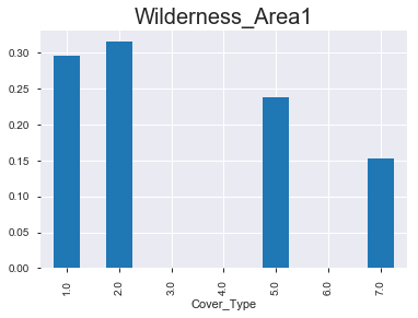
• 아래 그래프를 통해서 알 수 있 듯, 숲의 종류 마다 ‘wilderness area’가 매우 다름을 확인할 수 있다. 아직 모델링을 하지 않았지만, 뭔가 classification을 하는 데에 있어서 중요한 변수로 작용할 수 있다는 생각이 든다.

for i in train.columns[-45:-41]:
    plt.figure()
    ratio = pd.crosstab(train[i], train.Cover_Type, normalize='index').iloc[1,:].round(3)
    ratio.plot(kind='bar')
    plt.title(i, fontsize=20)
plt.show()

(2) 상대적 비율 & 절대적 값

• 위의 그래프를 수치로 확인해보면 다음과 같다.

for i in train.columns[-45:-41]:
    ratio = pd.crosstab(train[i], train.Cover_Type, normalize='index').iloc[1,:].round(3) # Cover_Type의 상대적 값 (비율)
    value = pd.crosstab(train[i], train.Cover_Type).iloc[1,:] # Cover_Type의 절대적 값 (개수)
    print("<",i,">")
    print(pd.concat([ratio,value],axis=1),'\n\n')

< Wilderness_Area1 >
              1.0   1.0
Cover_Type             
1.0         0.295  1062
2.0         0.315  1134
3.0         0.000     0
4.0         0.000     0
5.0         0.238   856
6.0         0.000     0
7.0         0.152   545 


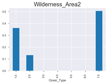
< Wilderness_Area2 >
              1.0  1.0
Cover_Type            
1.0         0.363  181
2.0         0.132   66
3.0         0.000    0
4.0         0.000    0
5.0         0.000    0
6.0         0.000    0
7.0         0.505  252 

    
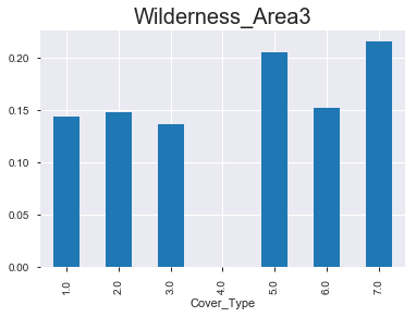
< Wilderness_Area3 >
              1.0   1.0
Cover_Type             
1.0         0.144   917
2.0         0.148   940
3.0         0.136   863
4.0         0.000     0
5.0         0.205  1304
6.0         0.152   962
7.0         0.215  1363 

   
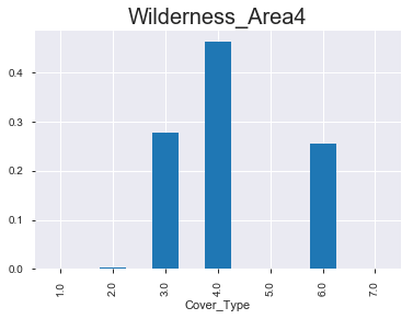
< Wilderness_Area4 >
              1.0   1.0
Cover_Type             
1.0         0.000     0
2.0         0.004    20
3.0         0.277  1297
4.0         0.462  2160
5.0         0.000     0
6.0         0.256  1198
7.0         0.000     0 

Q2. 토양 종류 (Soil_Type)에 따른 Cover_Type(Y값)은?

(1) Graph

for i in train.columns[-41:-1]:
    if (i != 'Soil_Type7') & (i!='Soil_Type15'):
        plt.figure()
        ratio = pd.crosstab(train[i], train.Cover_Type, normalize='index').iloc[1,:].round(3)
        ratio.plot(kind='bar')
        plt.title(i, fontsize=20)
plt.show()

(2) 상대적 비율 & 절대적 값

for i in train.columns[-41:-1]:
    if (i != 'Soil_Type7') & (i!='Soil_Type15'):
        ratio = pd.crosstab(train[i], train.Cover_Type, normalize='index').iloc[1,:].round(3)
        value = pd.crosstab(train[i], train.Cover_Type).iloc[1,:]
        print("<",i,">")
        print(pd.concat([ratio,value],axis=1),'\n\n')

Q3. 그 외의 Numerical 변수들에 따른 Cover_Type(Y값)은?

for i in train.columns[0:9]:
    plt.figure()
    sns.boxplot(x=train.Cover_Type, y = train[i])
    plt.title(i, fontsize=20)
plt.show()

4. Modeling

• 사용할 4개의 모델 : 1) Decision Tree
  2) Random Forest
  3) LightGBM
  4) XGBoost

Train = train.iloc[:,:-1] 
Test = train.iloc[:,-1]
x_train,x_test,y_train,y_test = train_test_split(Train,Test, test_size=0.2,random_state=42)

x_train = x_train.reset_index(drop=True)
x_test = x_test.reset_index(drop=True)

y_train = y_train.reset_index(drop=True)
y_test = y_test.reset_index(drop=True)

X = x_train
y = y_train 

5-fold CV를 통해, validation dataset의 accuracy가 가장 높은 모델을 선택할 것이다.

Default

• hyperparameter tuning 이전
• 최고 성능을 보인 것은 LightGBM : 84.38%이었다.

names = ['DecisionTree', 'RandomForest', 'LGBM', 'XGB']
clf_list = [DecisionTreeClassifier(random_state=42), RandomForestClassifier(random_state=42), lgb.LGBMClassifier(random_state=42), xgb.XGBClassifier(objective = 'multi:softprob',random_state=42) ]

for name, clf in zip(names, clf_list):
    clf.fit(X,y)
    print('---- {} ----'.format(name))
    print('cv score : ', cross_val_score(clf, X, y, cv=5).mean())

---- DecisionTree ----
cv score :  0.7683527742073142
---- RandomForest ----
cv score :  0.8197792619059616
---- LGBM ----
cv score :  0.8438330690017872
---- XGB ----
cv score :  0.7504086609575861

Hyperparameter Tuning

• 최적의 hyperparameter를 찾기 위해, 두 가지 방식 (Grid Search & Random Search)을 사용하였다.

from scipy.stats import randint
from sklearn.model_selection import GridSearchCV, RandomizedSearchCV

def hypertuning_rscv(est, p_distr, nbr_iter,X,y):
    rdmsearch = RandomizedSearchCV(est, param_distributions=p_distr, n_jobs=-1, n_iter=nbr_iter, cv=5, random_state=0)
    #CV = Cross-Validation ( here using Stratified KFold CV)
    rdmsearch.fit(X,y)
    ht_params = rdmsearch.best_params_
    ht_score = rdmsearch.best_score_
    return ht_params, ht_score

def hypertuning_gscv(est, p_distr,X,y):
    gdsearch = GridSearchCV(est, param_grid=p_distr, n_jobs=-1, cv=5)
    gdsearch.fit(X,y)
    bt_param = gdsearch.best_params_
    bt_score = gdsearch.best_score_    
    return bt_param, bt_score

dt_params = {"criterion": ["gini", "entropy"],
              "min_samples_split": randint(2, 20),
              "max_depth": randint(1, 20),
              "min_samples_leaf": randint(1, 20),
              "max_leaf_nodes": randint(2, 20)}

rf_params = {'max_depth':np.arange(3, 30), 
            'n_estimators':np.arange(100, 400),
            'min_samples_split':np.arange(2, 10)}

lgbm_params ={'max_depth': np.arange(3, 30),
             'num_leaves': np.arange(10, 100), 
             'learning_rate': [ 0.01, 0.05, 0.01, 0.001],
             'min_child_samples': randint(2, 30),
             'min_child_weight': [1e-5, 1e-3, 1e-2, 1e-1, 1, 1e1, 1e2, 1e3, 1e4],
             'subsample': np.linspace(0.6, 0.9, 30, endpoint=True), 
             'colsample_bytree': np.linspace(0.1, 0.8, 100, endpoint=True),
             'reg_alpha': [0, 1e-1, 1, 2, 5, 7, 10, 50, 100],
             'reg_lambda': [0, 1e-1, 1, 5, 10, 20, 50, 100],
             'n_estimators': np.arange(100, 400)}

xgb_params = {'eta':  np.linspace(0.001, 0.4, 50),
              'min_child_weight': [1, 5, 10],
              'gamma': np.arange(0, 20),
              'subsample': [0.6, 0.8, 1.0],
              'colsample_bytree': [0.6, 0.8, 1.0],
              'max_depth': np.arange(1, 500)}

params_list = [dt_params, rf_params, lgbm_params, xgb_params]

각 모델 별로 최적의 hyperparameter값을 best_param_dict에 넣는다.

best_param_dict = dict()
print('5-fold cross validation scores & best parameters :\n')
for name, clf, param_list in zip(names, clf_list, params_list):
    print('---- {} with RandomSearch ----'.format(name))
    
    best_params = hypertuning_rscv(clf, param_list, 30, X, y)
    best_param_dict[name] = best_params[0]
    print('best_params : ', best_params[0])
    
    clf.set_params(**best_params[0])
    cv_score = cross_val_score(clf, X, y, cv=5).mean()
    print('cv score : ', cv_score)

그 결과는 아래와 같다.

• 이번에는 RandomForest가 84.95%로 가장 좋은 성능을 보였다.
• 최적의 hyperparameter :
  • n_estimator (분류기의 개수) : 391
  • min_samples_split (분기가 일어나기 위한 최소한의 sample 개수) : 2
  • max_depth (tree의 최대 깊이) : 22

5-fold cross validation scores & best parameters :
---- DecisionTree with RandomSearch ----
best_params :  {'criterion': 'gini', 'max_depth': 18, 'max_leaf_nodes': 17, 'min_samples_leaf': 5, 'min_samples_split': 11}
cv score :  0.647404544674101
---- RandomForest with RandomSearch ----
best_params :  {'n_estimators': 391, 'min_samples_split': 2, 'max_depth': 22}
cv score :  0.8495366799306494
---- LGBM with RandomSearch ----
best_params :  {'colsample_bytree': 0.4747474747474748, 'learning_rate': 0.05, 'max_depth': 9, 'min_child_samples': 10, 'min_child_weight': 1, 'n_estimators': 373, 'num_leaves': 89, 'reg_alpha': 5, 'reg_lambda': 0.1, 'subsample': 0.7034482758620689}
cv score :  0.8291166436732764
---- XGB with RandomSearch ----
best_params :  {'subsample': 0.6, 'min_child_weight': 5, 'max_depth': 356, 'gamma': 0, 'eta': 0.20457142857142857, 'colsample_bytree': 0.8}
cv score :  0.8467260432797161

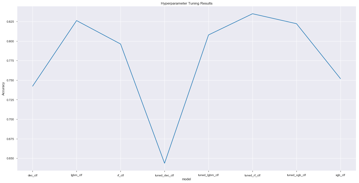
총 8개의 모델의 성능을 보면 다음과 같다. (tuning 이전 4개 + tuning 이후 4)

names = ['dec_clf', 'rf_clf','lgbm_clf','xgb_clf','tuned_dec_clf','tuned_rf_clf','tuned_lgbm_clf',
         'tuned_xgb_clf']

labels = ['DecisionTree', 'RandomForest', 'LGBM','XGB',
       'Tuned_DecisionTree', 'Tuned_RandomForest', 'Tuned_LGBM','Tuned_XGB']

clf_list = [DecisionTreeClassifier(random_state=42),
            RandomForestClassifier(random_state=42),
            lgb.LGBMClassifier(random_state=42),
            xgb.XGBClassifier(random_state=42),
            
            DecisionTreeClassifier(random_state=42, **best_param_dict['DecisionTree']),
            RandomForestClassifier(random_state=42, **best_param_dict['RandomForest']),
            lgb.LGBMClassifier(random_state=42, **best_param_dict['LGBM']),
            xgb.XGBClassifier(random_state=42, **best_param_dict['XGB'])]

scores_list = dict()
for name, label, clf in zip(names, labels, clf_list):
    print('---- {} ----'.format(name))
    scores = cross_val_score(clf, X, y, cv=2, scoring='accuracy')
    scores_list[name] = scores[0]
    print ("Accuracy: %.2f (+/- %.2f) [%s]" %(scores.mean(), scores.std(), label))
    
plt.figure(figsize=(20,10))
plt.plot(*zip(*sorted(scores_list.items())))
plt.ylabel('Accuracy'); plt.xlabel('model'); plt.title('Hyperparameter Tuning Results');
plt.show()

---- dec_clf ----
Accuracy: 0.74 (+/- 0.00) [DecisionTree]
---- rf_clf ----
Accuracy: 0.79 (+/- 0.01) [RandomForest]
---- lgbm_clf ----
Accuracy: 0.82 (+/- 0.00) [LGBM]
---- xgb_clf ----
Accuracy: 0.75 (+/- 0.01) [XGB]
---- tuned_dec_clf ----
Accuracy: 0.65 (+/- 0.00) [Tuned_DecisionTree]
---- tuned_rf_clf ----
Accuracy: 0.83 (+/- 0.01) [Tuned_RandomForest]
---- tuned_lgbm_clf ----
Accuracy: 0.80 (+/- 0.01) [Tuned_LGBM]
---- tuned_xgb_clf ----
Accuracy: 0.82 (+/- 0.01) [Tuned_XGB]

Stacking

지금 까지 만든 모델들을 사용해서 Stacking을 해보았다. Meta Learner로는 Logistic Regression을 사용하였다.

from mlxtend.classifier import StackingCVClassifier
from sklearn.linear_model import LinearRegression, LogisticRegression
lr = LogisticRegression()
ens_dt = BaggingClassifier(DecisionTreeClassifier(random_state=42),oob_score=True,random_state=42)
ens_rf = RandomForestClassifier(random_state=42, **best_param_dict['RandomForest'])
ens_lgbm = lgb.LGBMClassifier(random_state=42, **best_param_dict['LGBM'])
#ens_xbg_model = xgb.XGBClassifier(random_state=42, **best_param_dict['XGB'])

stack = StackingCVClassifier(classifiers=(ens_dt, ens_rf, ens_lgbm),
                            meta_classifier=ens_rf,random_state=42)

print('5-fold cross validation score:\n')
print('---- {} ----'.format('Stacking Model'))
cv_score = cross_val_score(stack, X, y, cv=5).mean()
print('cv_score :', cv_score)

5-fold cross validation score:

---- Stacking Model ----
cv_score : 0.8485440203329828

---

[ 부록 ]

Classification Using Neural Network

머신러닝 모델 말고, 딥러닝을 이용하여 분류도 해보았다. 차이점은, input으로 넣을 때 전부 scaling을 해줬다는 점이다. (neuralnet의 경우에는 feature의 scale에 민감하므로)

1. Importing Data

import pandas as pd
import numpy as np

train = pd.read_csv('train.csv')

train.drop('Id', axis=1, inplace=True)

2. Scaling data

from sklearn.preprocessing import StandardScaler
from sklearn.model_selection import train_test_split

sc = StandardScaler()

def scalingcolumns(df, cols_to_scale):
    for col in cols_to_scale:
        df[col] = pd.DataFrame( sc.fit_transform(pd.DataFrame(train[col])),columns=[col] )
    return df

cols_to_scale = train.columns[0:-1]
scaled_data = scalingcolumns(train,cols_to_scale)

scaled_data_x = scaled_data.iloc[:,:-1]
scaled_data_y = scaled_data.iloc[:,-1]

scaled_data_y = scaled_data_y-1

• train과 test는 8:2로 나누었다.

x_train,x_test,y_train,y_test = train_test_split(scaled_data_x,scaled_data_y, test_size=0.2,random_state=42)

3. Modeling

import torch
from torch.autograd import Variable
import torchvision.transforms as transforms
import torch.nn.init
import torch.nn as nn
import torch.utils.data as data_utils

# setting hyper parameter
lr = 0.02
training_epochs = 400
batch_size = 288
#keep_prob = 0.7

train.shape

(15120, 55)

trainx = torch.tensor(x_train.values.astype(np.float32))
trainy = torch.tensor(y_train.values)

train_tensor = data_utils.TensorDataset(trainx, trainy) 

train_loader = data_utils.DataLoader(dataset = train_tensor, batch_size = batch_size, shuffle = True)

• 다음과 같은 4개의 layer를 쌓았다.

linear1 = nn.Linear(54, 54, bias=True)
linear2 = nn.Linear(54, 54, bias=True)
linear3 = nn.Linear(54, 54, bias=True)
linear4 = nn.Linear(54, 7, bias=True)

• batch normalization

bn1 = nn.BatchNorm1d(54)
bn2 = nn.BatchNorm1d(54)
bn3 = nn.BatchNorm1d(54)
bn4 = nn.BatchNorm1d(7)

relu = nn.ReLU()

# BN으로 이미 regularization 충분!
#dropout = nn.Dropout(p=1 - keep_prob)

• weight의 초기값으로는 He초기값을 사용하였다. ( nn.init.kaiming_uniform )

nn.init.kaiming_uniform_(linear1.weight, mode='fan_in', nonlinearity='relu')
nn.init.kaiming_uniform_(linear2.weight, mode='fan_in', nonlinearity='relu')
nn.init.kaiming_uniform_(linear3.weight, mode='fan_in', nonlinearity='relu')
nn.init.kaiming_uniform_(linear4.weight, mode='fan_in', nonlinearity='relu')

#nn.init.xavier_uniform_(linear1.weight)
#nn.init.xavier_uniform_(linear2.weight)
#nn.init.xavier_uniform_(linear3.weight)
#nn.init.xavier_uniform_(linear4.weight)

• 마지막에는 multi-class classification을 위해 Softmax Function을 사용하였다

model = nn.Sequential(linear1, bn1, relu,
                                     linear2, bn2, relu,
                                     linear3, bn3, relu,
                                     linear4, bn4, nn.Softmax())

• Loss Function으로는 Cross Entropy를, Optimizer로는 Adam을 사용하였다.

criterion = nn.CrossEntropyLoss()
optimizer = torch.optim.Adam(model.parameters(), lr=lr)

for epoch in range(training_epochs):
    avg_cost = 0
    total_batch = x_train.shape[0] // batch_size
    
    for i, (batch_xs, batch_ys) in enumerate(train_loader):
        X = Variable(batch_xs.view(288,54))
        Y = Variable(batch_ys)
        
        optimizer.zero_grad()
        hypothesis = model(X)
        cost = criterion(hypothesis, Y.long())
        cost.backward()
        optimizer.step()
        
        avg_cost += cost/total_batch
    
    if epoch%10==0:
        print("[Epoch: {:>4}] cost = {:>.9}".format(epoch, avg_cost.data))

[Epoch:    0] cost = 1.72366369
[Epoch:   10] cost = 1.38898396
[Epoch:   20] cost = 1.35898578
[Epoch:   30] cost = 1.34380758
[Epoch:   40] cost = 1.33171129
[Epoch:   50] cost = 1.32044339
...
[Epoch:  360] cost = 1.24475861
[Epoch:  370] cost = 1.24499512
[Epoch:  380] cost = 1.24003696
[Epoch:  390] cost = 1.2397511

testx = torch.tensor(x_test.values.astype(np.float32))
testy = torch.tensor(y_test.values)

4. Result

(1) train accuracy

trainpred = model(trainx)

correct_trainpred = torch.max(trainpred.data, 1)[1] == trainy.data
correct_trainpred

tensor([1, 1, 1,  ..., 1, 1, 1], dtype=torch.uint8)

trainacc = correct_trainpred.float().mean()
print("Accuracy :", trainacc)

Accuracy : tensor(0.9396)

(2) test accuracy

pred = model(testx)

correct_pred = torch.max(pred.data, 1)[1] == testy.data
correct_pred

tensor([1, 0, 1,  ..., 1, 1, 1], dtype=torch.uint8)

accuracy = correct_pred.float().mean()
print("Accuracy :", accuracy)

Accuracy : tensor(0.8644)

Overfitting이 발생한 것으로 보인다. 이를 해결하기 위해 drop out도 사용해봤지만, 오히려 성능이 더 좋지 않게 나왔다.