(Diffusion survey) (Part 1; xxx)

Diffusion Models and Representation Learning: A Survey

https://arxiv.org/pdf/2407.00783

Contents

Abstract

Diffusion Models

• Popular generative modeling methods
• Unique instance of SSL methods (due to their independence from label annotation)

This paper:

• Explores the interplay between (1) diffusion models and (2) representation learning
• Overview of diffusion models’ essential aspects, including ..
  • (1) Mathematical foundations
  • (2) Popular denoising network architectures
  • (3) Guidance methods
• Frameworks that leverage representations learned from pre-trained diffusion models for subsequent recognition tasks
• Methods that utilize advancements in SSL to enhance diffusion models
• Comprehensive overview of the taxonomy between diffusion models and representation learning

1. Introduction

P1) Intro to diffusion models

Recently emerged as the SOTA of generative modeling

P2) SSL

Scalability

• Current SOTA SSL show great scalability!
• Diffusion models exhibit similar scaling properties

Generation

• Controlled generation approaches

  • e.g., Classifier Guidance [43] and Classifier-free Guidance [67]
    • Rely on annotated data \(\rightarrow\) Bottleneck for scaling up!

• Guidance approaches that leverage “representation learning”

  \(\rightarrow\) Potentially enabling diffusion models to train on much larger, annotation-free datasets.

P3) Diffusion & representation learning

Two central perspectives

• (1) Using diffusion models themselves for representation learning
• (2) Using representation learning for improving diffusion models.

P4) Increasing works

P5)

Current approaches:

\(\rightarrow\) Rely on using diffusion models solely trained for generative synthesis for representation learning.

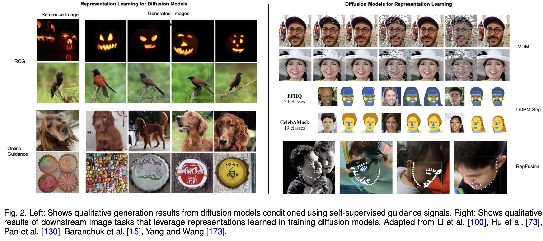
Qualitative results

P6) Main contributions

• (1) Comprehensive Overview
  • Interplay between diffusion models and representation learning
  • How diffusion models can be used for representation learning and vice versa
• (2) Taxonomy of Approaches
  • Approaches in diffusion-based representation learning
• (3) Generalized Frameworks
  • Generalized frameworks for both …
    • (1) diffusion model feature extraction
    • (2) assignment-based guidance
• (4) Future Directions

2. Background

The following section outlines the required mathematical foundations of diffusion models. We also highlight current architecture backbones of diffusion models and provide a brief overview of sampling methods and conditional generation approaches.

(1) Mathematical Foundations

a) Forward process

\(\begin{gathered} p\left(\mathbf{x}_t \mid \mathbf{x}_{t-1}\right)=\mathcal{N}\left(\mathbf{x}_t ; \sqrt{1-\beta_t} \mathbf{x}_{t-1}, \quad \beta_t \mathbf{I}\right), \\ \forall t \in\{1, \ldots, T\} \end{gathered}\).

\(p\left(\mathbf{x}_t \mid \mathbf{x}_0\right)=\mathcal{N}\left(\mathbf{x}_t ; \sqrt{\bar{\alpha}_t} \mathbf{x}_0 ;\left(1-\bar{\alpha}_t\right) \mathbf{I}\right)\).

• where \(\alpha_t:=1-\beta_t\) and \(\bar{\alpha}_t:=\prod_{i=1}^t \alpha_i\).

\(\mathbf{x}_t=\sqrt{\bar{\alpha}_t} \mathbf{x}_0+\sqrt{\left(1-\bar{\alpha}_t\right)} \epsilon_t\).

b) Backward process

\(\mathbf{x}_T \sim \pi\left(\mathbf{x}_T\right)=\mathcal{N}(0, \mathbf{I})\) .

\(p_\theta\left(\mathbf{x}_{t-1} \mid \mathbf{x}_t\right)= \mathcal{N}\left(\mathbf{x}_{t-1} ; \mu_\theta\left(\mathbf{x}_t, t\right), \Sigma_\theta\left(\mathbf{x}_t, t\right)\right)\).

c) Loss function

\(\begin{aligned} \mathcal{L}_{v t b}= & -\log p_\theta\left(\mathbf{x}_0 \mid \mathbf{x}_1\right)+D_{K L}\left(p\left(\mathbf{x}_T \mid \mathbf{x}_0\right) \mid \mid \pi\left(\mathbf{x}_T\right)\right) \\ & +\sum_{t>1} D_{K L}\left(p\left(\mathbf{x}_{t-1} \mid \mathbf{x}_t, \mathbf{x}_0\right) \mid \mid p_\theta\left(\mathbf{x}_{t-1} \mid \mathbf{x}_t\right)\right) \end{aligned}\).

d) Mean & Noise prediction

\(\mu\left(\mathbf{x}_t, t\right):=\frac{\sqrt{\alpha_{t-1}}\left(1-\bar{\alpha}_{t-1}\right) \mathbf{x}_t+\sqrt{\bar{\alpha}_{t-1}}\left(1-\alpha_t\right) \mathbf{x}_0}{1-\bar{\alpha}_t}\).

\(\mu_\theta\left(\mathbf{x}_t, t\right)=\frac{1}{\sqrt{\alpha_t}}\left(\mathbf{x}_t-\frac{1-\alpha_t}{\sqrt{1-\bar{\alpha}_t}} \boldsymbol{\epsilon}_\theta\left(\mathbf{x}_t, t\right) .\right)\).

• DDPM:
  • Suggest fixing the covariance \(\Sigma_\theta\left(\mathbf{x}_t, t\right)\) to a constant value
  • Suggest predicting the added noise \(\boldsymbol{\epsilon}\left(\mathbf{x}_t, t\right)\) instead of \(\mathbf{x}_0\)
• Loss function becomes…
  • \(\mathcal{L}_{\text {simple }}=\mathbb{E}_{t \sim[1, T]} \mathbb{E}_{\mathbf{x}_0 \sim p\left(\mathbf{x}_0\right)} \mathbb{E}_{\boldsymbol{\epsilon}_{\mathrm{t}} \sim \mathcal{N}(0, \mathbf{I})} \mid \mid \boldsymbol{\epsilon}_{\mathrm{t}}-\boldsymbol{\epsilon}_\theta\left(\mathbf{x}_t, t\right) \mid \mid ^2\).

e) Improving sampling efficiency

Velocity prediction

• Velocity = Linear combination of the denoised input & the added noise
• \(\mathbf{v}=\bar{\alpha}_t \epsilon-\left(1-\bar{\alpha}_t\right) \mathbf{x}_t\).

\(\rightarrow\) Combines benefits of both data and noise parametrizations

f) Stochastic Differential Equation (SDE)

Continuous (O) Discrete (X) timeseteps

Diffusion process = Continuous time-dependent function \(\sigma(t)\).

\(d \mathbf{x}=\mathbf{f}(\mathbf{x}, t) d t+g(t) d \mathbf{w}\).

• Vector-valued drift coefficient \(\mathbf{f}(\cdot, t): \mathbb{R}^d \rightarrow \mathbb{R}^d\)
• Scalar-valued diffusion coefficient \(g(\cdot): \mathbb{R} \rightarrow \mathbb{R}\)
• \(\mathbf{w}\): standard Wiener process

Two widely used choices of the SDE formulation

\(\rightarrow\) Differs by the assumption of the drift term and diffusion term!

• (1) Variance-Preserving (VP) SDE
• (2) Variance-Exploding (VE) SDE

(1) Variance-Preserving (VP) SDE

• Drift: \(\mathbf{f}(\mathbf{x}, t)=-\frac{1}{2} \beta(t) \mathbf{x}\).
• Diffusion: \(g(t)=\sqrt{\beta(t)}\)
• Equivalent to the continuous formulation of the DDPM parametrization

(2) Variance-Exploding (VE) SDE

• Drift: \(\mathbf{f}(\mathbf{x}, t)=0\)
• Diffusion: \(g(t)=\sqrt{2 \alpha(t) {d t}} =\sqrt{2 \sigma(t) \frac{d \sigma(t)}{d t}}\)
• Variance continually increases with increasing \(t\)
• Widely used in score-based models

Type	Drift Term (\(f(x,t)\mathbf{f}(\mathbf{x}, t)\))	Diffusion Term (g(t)g(t))	Example
VP SDE	\(-\frac{1}{2} \beta(t) \mathrm{x}\)	\(\sqrt{\beta(t)}\)	\(\beta(t)=\beta_{\min }+\left(\beta_{\max }-\beta_{\min }\right) t\)
VE SDE	\(0\)	\(\sqrt{2 \alpha(t)}\)	\(\alpha(t)=\alpha_{\min }\left(\alpha_{\max } / \alpha_{\min }\right)^t\)

Summary 1) General

• Forward SDE: \(d \mathbf{x}=\mathbf{f}(\mathbf{x}, t) d t+g(t) d \mathbf{w}\).

• Reverse SDE: \(d \mathbf{x}=\left[\mathbf{f}(\mathbf{x}, t)-g(t)^2 \nabla_{\mathbf{x}} \log p_t(\mathbf{x})\right] d t+g(t) d \mathbf{w}\).

  • \(\nabla_{\mathbf{x}} \log p(\mathbf{x} ; \sigma(t))\) = Score function

    \(\rightarrow\) Generally not known! Approximated using a NN!

Summary 2) VP-SDE

• Forward SDE:
  • \(\begin{aligned} d \mathbf{x}&=\mathbf{f}(\mathbf{x}, t) d t+g(t) d \mathbf{w}\\&=-\frac{1}{2} \beta(t) \mathbf{x} d t+ \sqrt{\beta(t)} d \mathbf{w}\end{aligned}\).
• Reverse SDE:
  • \(\begin{aligned}d \mathbf{x}&=\left[\mathbf{f}(\mathbf{x}, t)-g(t)^2 \nabla_{\mathbf{x}} \log p_t(\mathbf{x})\right] d t+g(t) d \mathbf{w}\\&= \left[-\frac{1}{2} \beta(t) \mathbf{x}- \beta(t) \nabla_{\mathbf{x}} \log p_t(\mathbf{x})\right] d t+ \sqrt{\beta(t)} d \mathbf{w}\end{aligned}\).

Summary 3) VE-SDE

• Forward SDE:
  • \(\begin{aligned}d \mathbf{x}&=\mathbf{f}(\mathbf{x}, t) d t+g(t) d \mathbf{w}\\&= \sqrt{2 \sigma(t) \frac{d \sigma(t)}{d t}}d \mathbf{w}\end{aligned}\).
• Reverse SDE:
  • \(\begin{aligned} d \mathbf{x}&=\left[\mathbf{f}(\mathbf{x}, t)-g(t)^2 \nabla_{\mathbf{x}} \log p_t(\mathbf{x})\right] d t+g(t) d \mathbf{w} \\& =-2 \sigma(t) \frac{d \sigma(t)}{d t} \nabla_{\mathbf{x}} \log p_t(\mathbf{x}) d t+\sqrt{2 \sigma(t) \frac{d \sigma(t)}{d t}} d \mathbf{w}\end{aligned}\).

(2) Backbone Architectures

Denoising prediction networks (parameters \(\theta\))

Discuss the formulation of \(\theta\) by several NN architectures

• To approximate the score function

• Map from the same input space to the same output space

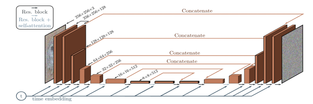
a) U-Net

[1] DDPM

• U-Net backbone (similar to an unmasked PixelCNN++)
  • Originally used in semantic segmentation

• DDPMs: Operate in the pixel space

  \(\rightarrow\) Training and inference: computationally expensive

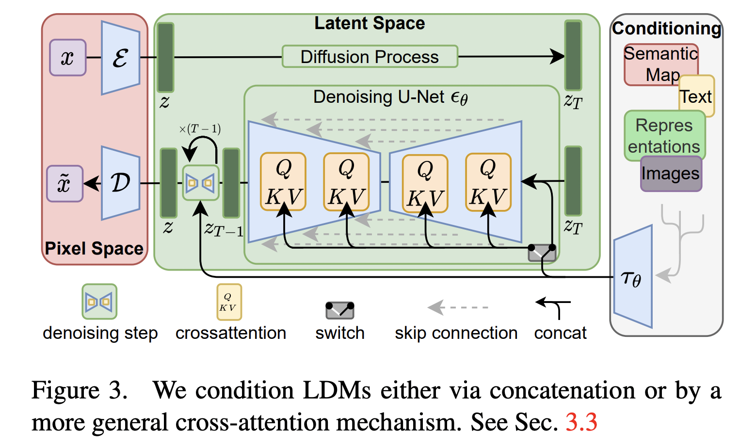
[2] Latent Diffusion Models (LDMs)

• Operate in the latent space of a pre-trained VAE

  ( = Diffusion process is applied to the generated representation (instead of pixel space))

  \(\rightarrow\) Computational benefits without sacrificing generation quality!

• Architecture: U-Net + Additional cross-attention

  • For more flexible conditioned generation

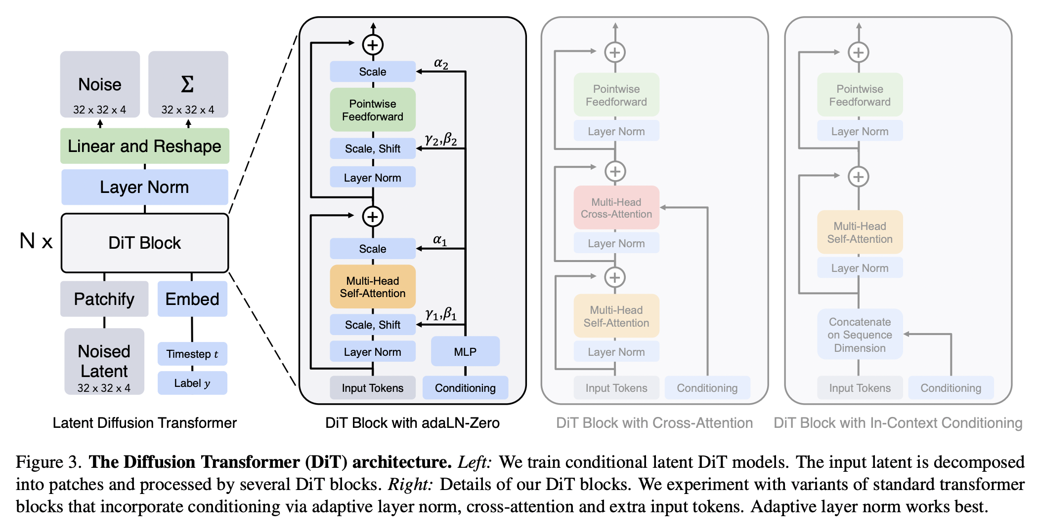
b) Transformer (e.g., ViT)

[1] Diffusion Transformers (DiT)

• Largely inspired by ViTs
  • Transform input images into a sequence of patches!

• Demonstrates SOTA generation performance on ImageNet when combined with the LDM

• Details
  • Into a sequence of tokens using a “patchify” layer
  • Add ViT-style positional embeddings to all input tokens

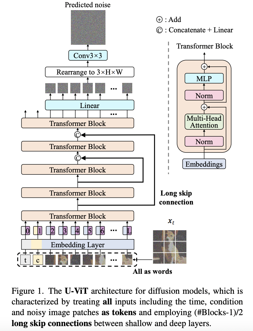
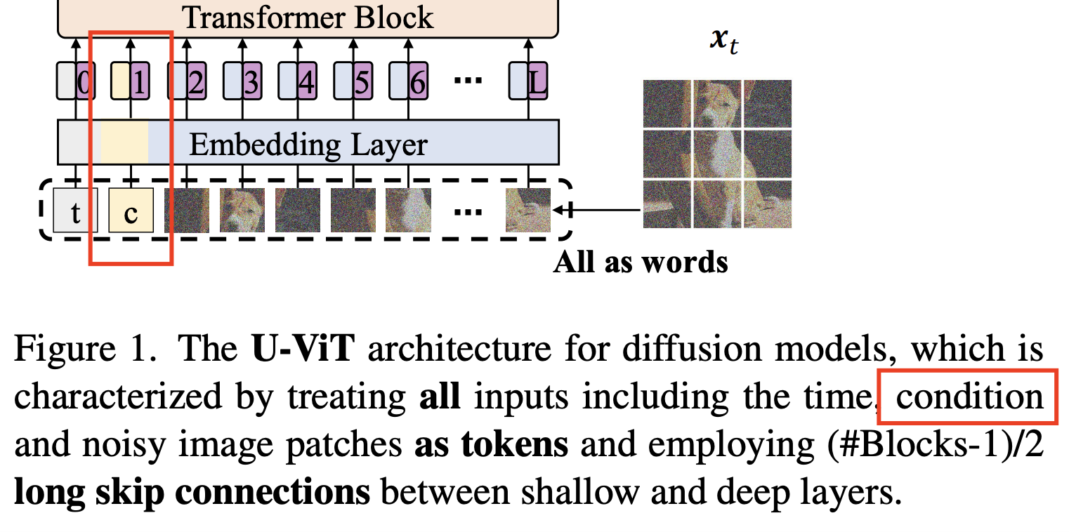
[2] U-ViTs

• Unified backbone (U-Net + ViT)

  • (1) ViT: Design methodology of transformers in tokenizing time, conditioning and image inputs

  • (2) U-Net: Additionally employ long skip connections between shallow and deep layers

    \(\rightarrow\) Provide shortcuts for low-level features \(\rightarrow\) Stabilize training of the denoising network

• Results: On par with U-Net CNN-based architectures!

(3) Diffusion Model Guidance

Recent improvements in image generation:

\(\rightarrow\) By improved guidance approaches!

• Ability to control generation by passing user-defined conditions
• Guidance = modulation of the strength of the conditioning signal within the model

a) Conditioning signals

• Wide range of modalities
  • e.g., Class labels, text embeddings to other images….
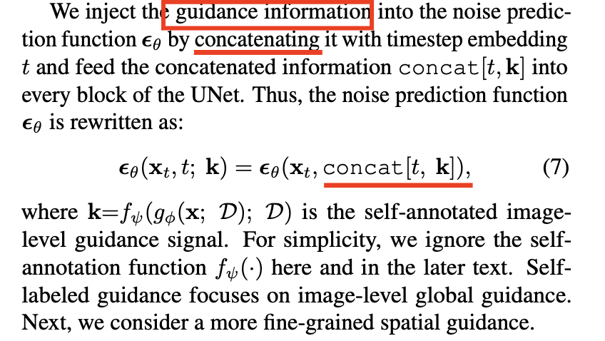
• Method 1) Naive way
  • Concatenate the conditioning signal with the denoising targets
  • Then pass the signal through the denoising network
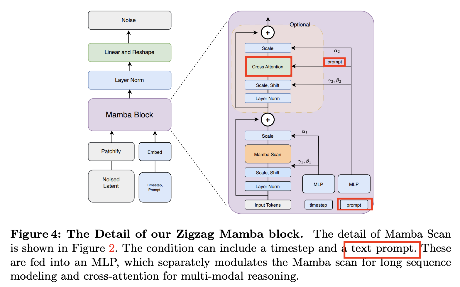
• Method 2) Cross-attention
  • Conditioning signal \(\mathbf{c}\) is preprocessed by an encoder to an intermediate projection \(E(c)\)
  • Then injected into the intermediate layer of the denoising network using cross-attention
  • [76, 142]. These conditioning approaches alone do not leave the possibility

Method 1) Naive way

Method 2) Cross-attention

b) Classifier guidance (CG)

Compute-efficient method

How? Leveraging a (pre-trained) noise robust classifier

• Idea: Can be conditioned using the gradients of a classifier \(p_\phi\left(\mathbf{c} \mid \mathbf{x}_{\mathbf{t}}, t\right)\).

Gradients of the \(\log\)-likelihood of this classifier: \(\nabla_{\mathbf{x}_{\mathbf{t}}} \log p_\phi\left(\mathbf{c} \mid \mathbf{x}_{\mathbf{t}}, t\right)\)

\(\rightarrow\) Guide the diffusion process towards generating an image belonging to class label \(\mathbf{c}\).

Mathematical expressions

• Score estimator for \(p(x \mid c)\) :
  • \(\nabla_{\mathbf{x}_{\mathbf{t}}} \log \left(p_\theta\left(\mathbf{x}_{\mathbf{t}}\right) p_\phi\left(\mathbf{c} \mid \mathbf{x}_{\mathbf{t}}\right)\right)=\nabla_{\mathbf{x}_{\mathbf{t}}} \log p_\theta\left(\mathbf{x}_{\mathbf{t}}\right)+\nabla_{\mathbf{x}_{\mathbf{t}}} \log p_\phi\left(\mathbf{c} \mid \mathbf{x}_{\mathbf{t}}\right)\).
• Noise prediction network:
  • \(\hat{\epsilon}_\theta\left(\mathbf{x}_{\mathbf{t}}, \mathbf{c}\right)=\epsilon_\theta\left(\mathbf{x}_{\mathbf{t}}, \mathbf{c}\right)-w \sigma_t \nabla_{\mathbf{x}_{\mathbf{t}}} \log p_\phi\left(\mathbf{c} \mid \mathbf{x}_{\mathbf{t}}\right)\).
    • where the parameter \(w\) modulates the strength of the conditioning signal.

Summary

• Classifier guidance is a versatile approach that increases sample quality!

• But it is heavily reliant on the availability of a noise-robust pre-trained classifier

  \(\rightarrow\) Relies on the availability of annotated data

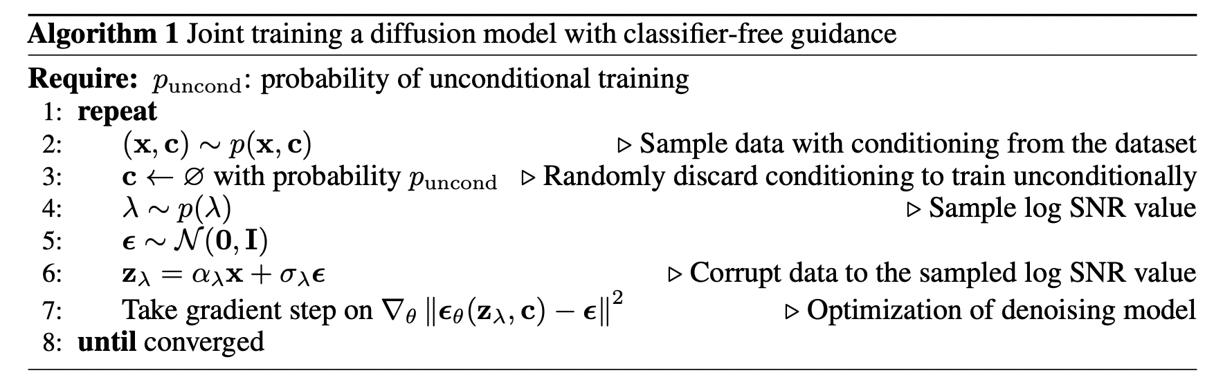
c) Classifier-free guidance (CFG)

Eliminates the need for a pre-trained classifier!

How? Single model \(\epsilon_\theta\left(\mathbf{x}_{\mathbf{t}}, t, \mathbf{c}\right)\).

• (1) Unconditional: \(\mathbf{c} = \phi\)
  • Randomly dropping out the conditioning signal with probability \(p_{\text {uncond }}\).
• (2) Conditional: \(\mathbf{c}\)

Sampling

• Weighted combination of conditional and unconditional score estimates

• \(\tilde{\epsilon}_\theta\left(\mathbf{x}_{\mathbf{t}}, \mathbf{c}\right)=(1+w) \epsilon_\theta\left(\mathbf{x}_{\mathbf{t}}, \mathbf{c}\right)-w \epsilon_\theta\left(\mathbf{x}_{\mathbf{t}}, \phi\right)\).

• Does not rely on the gradients of a pre-trained classifier!

  ( But still requires an annotated dataset to train the conditional denoising network )

CG vs. CFG

• (CG) \(\hat{\epsilon}_\theta\left(\mathbf{x}_{\mathbf{t}}, \mathbf{c}\right)=\epsilon_\theta\left(\mathbf{x}_{\mathbf{t}}, \mathbf{c}\right)-w \sigma_t \nabla_{\mathbf{x}_{\mathbf{t}}} \log p_\phi\left(\mathbf{c} \mid \mathbf{x}_{\mathbf{t}}\right)\).
• (CFG) \(\tilde{\epsilon}_\theta\left(\mathbf{x}_{\mathbf{t}}, \mathbf{c}\right)=(1+w) \epsilon_\theta\left(\mathbf{x}_{\mathbf{t}}, \mathbf{c}\right)-w \epsilon_\theta\left(\mathbf{x}_{\mathbf{t}}, \phi\right)\).

d) Summary

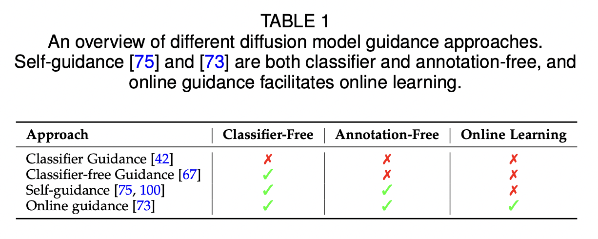
Classifier and classifier-free guidance

\(\rightarrow\) Controlled generation methods

Fully unconditional approaches?

• Recent works using diffusion model representations for SSL guidance!
• Do not need annotated data

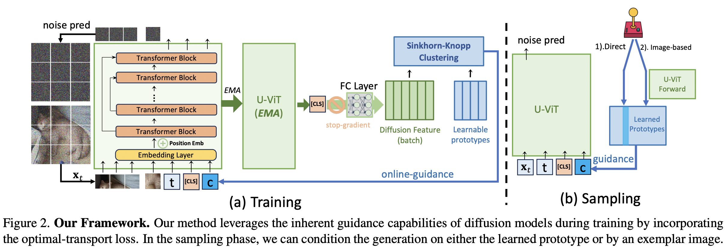
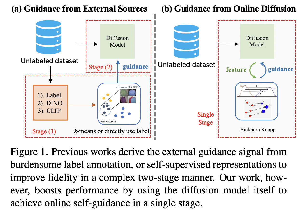
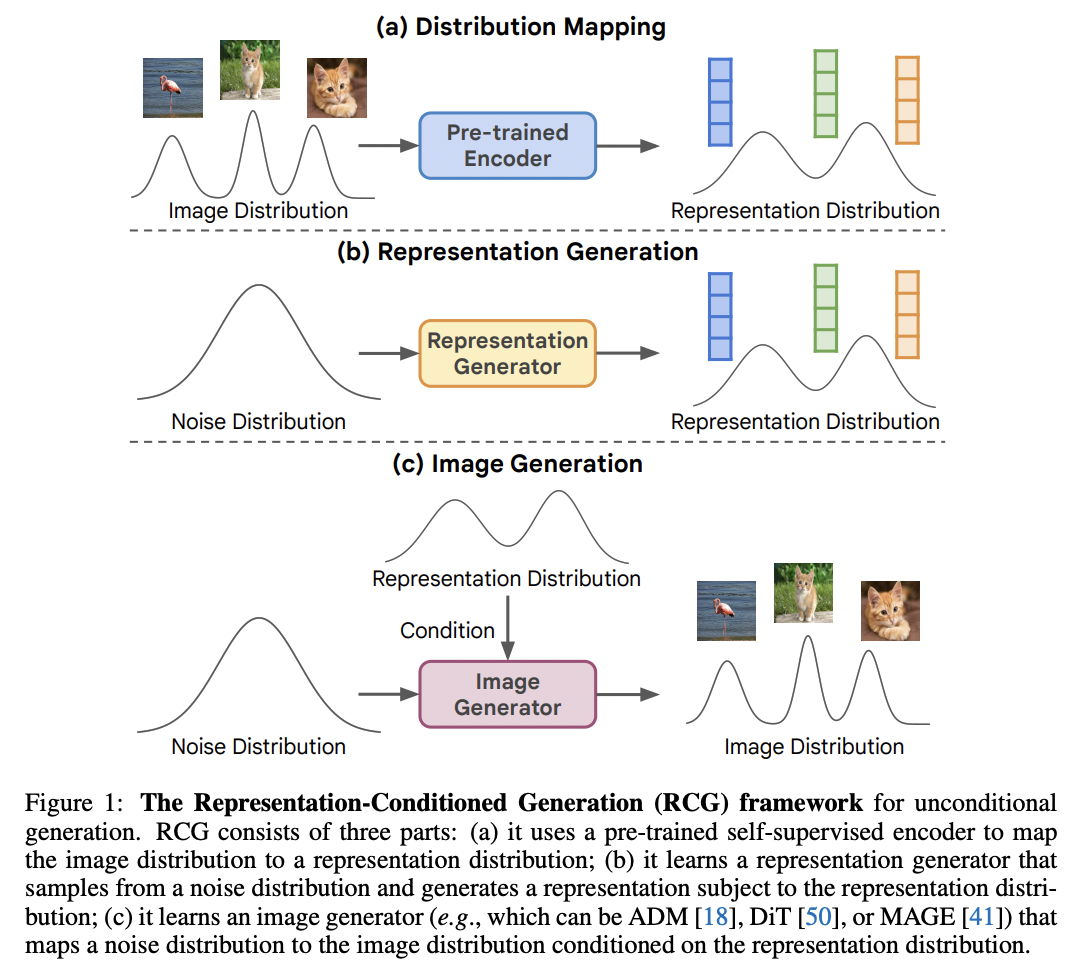
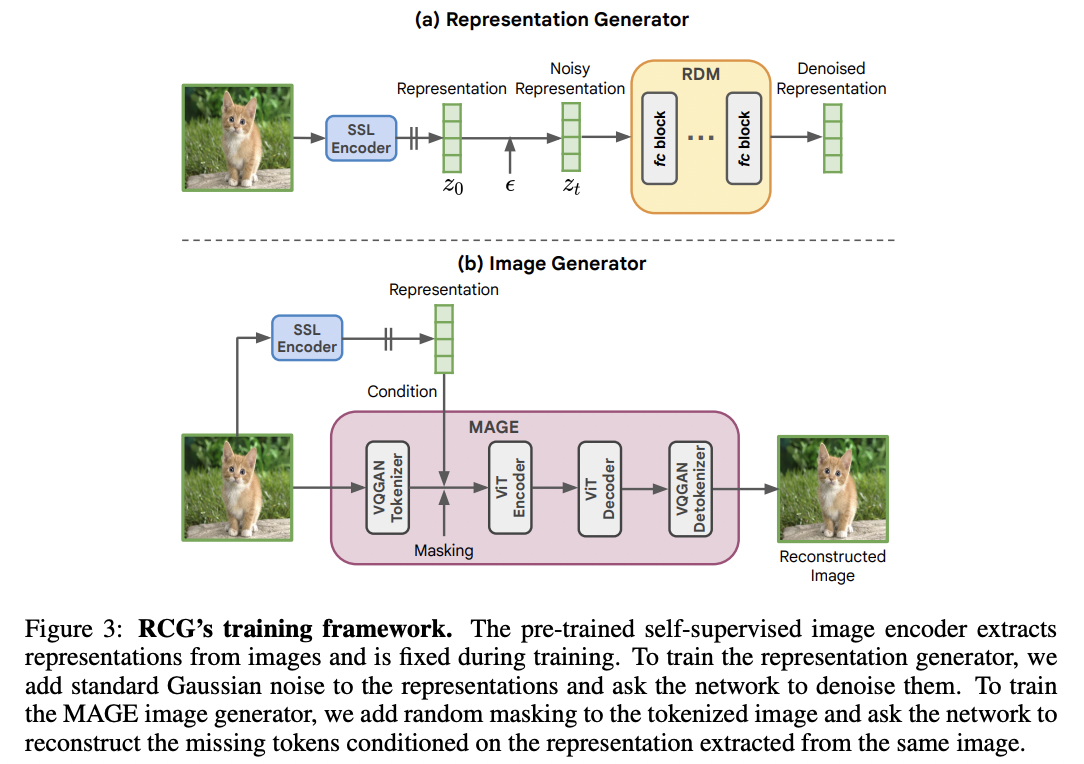
Representation-Conditioned Generation (RCG)