Context-Aware Self-Attention Networks (2019)
Contents
-
Abstract
-
Introduction
-
Background ( SANs )
-
기존의 SANs
- Motivation
- Approach
-
0. Abstract
Self-attention의 특징/장점
- flexibility in parallel computation
- long & short-term dependency 모두 잡아내
\(\rightarrow\) contextual information을 잡아내지는 X
따라서, 이 논문은 self-attention network (SAN)를 improve시킴!
( by capturing the CONTEXTUAL information )
HOW? contextualize the transformations of the QUERY and KEY layers
1. Introduction
SANs ( Self-attention networks )
-
Lin et al. 2017
-
장점 : long-range dependency도 포착 가능
-
문제점 : treat input sequence as bag-of-word tokens &
각각의 token INDIVIDUALLY performs attention
\(\rightarrow\) contextual information 반영 X
Propose to strengthen SANs through capturing the richness of context
2. Background ( SANs )
2-1) 기존의 SANs
“pair of token 사이의 attention weight를 계산한다”
-
Input Layer : \(\mathbf{H}=\left\{h_{1}, \ldots, h_{n}\right\}\)
- Q,K,V : \(\mathbf{H}\) 에 weight를 곱해서 얻어낸다. …. \(\left[\begin{array}{c} \mathbf{Q} \\ \mathbf{K} \\ \mathbf{V} \end{array}\right]=\mathbf{H}\left[\begin{array}{l} \mathbf{W}_{Q} \\ \mathbf{W}_{K} \\ \mathbf{W}_{V} \end{array}\right]\)
-
Output Layer : \(\mathrm{O}=\operatorname{ATT}(\mathbf{Q}, \mathbf{K}) \mathbf{V}\)
- Attention 2가지 방법
- 1) additive
- 2) dot-product \(\rightarrow\) 이거 사용! \(\operatorname{ATT}(\mathbf{Q}, \mathbf{K})=\operatorname{softmax}\left(\frac{\mathbf{Q K}^{T}}{\sqrt{d}}\right)\)
2-2) Motivation
\(Q\)와 \(V\) 사이의 similarity 계산 시… only 2 parameter matrices
- \(\mathbf{Q K}^{T}=\left(\mathbf{H W}_{Q}\right)\left(\mathbf{H W}_{K}\right)^{T}=\mathbf{H}\left(\mathbf{W}_{Q} \mathbf{W}_{K}^{T}\right) \mathbf{H}^{T}\).
2-3) Approach
여러 종류의 Context vector를 제안한다
( + 어떻게 SAN에 incorporate 시킬지 )
(a) Context-Aware Self-Attention Model
propose to contextualize the transformations from the input layer \(\mathbf{H}\) to Q & V
Shaw et al (2018)의 contextual information을 propagate하는 방법 차용
-
\(\left[\begin{array}{c} \widehat{\mathbf{Q}} \\ \widehat{\mathbf{K}} \end{array}\right]=\left(1-\left[\begin{array}{c} \lambda_{Q} \\ \lambda_{K} \end{array}\right]\right)\left[\begin{array}{l} \mathbf{Q} \\ \mathbf{K} \end{array}\right]+\left[\begin{array}{c} \lambda_{Q} \\ \lambda_{K} \end{array}\right]\left(\mathbf{C}\left[\begin{array}{c} \mathbf{U}_{Q} \\ \mathbf{U}_{K} \end{array}\right]\right)\).
where \(\mathbf{C} \in \mathbb{R}^{n \times d_{c}}\) is the context vector
where \(\left\{\mathbf{U}_{Q}, \mathbf{U}_{K}\right\} \in\) is a trainable parameter
\(\left\{\lambda_{Q}, \lambda_{K}\right\}\) : can also be treated as factors to regulate the magnitude of \(\widehat{Q}\) and \(\widehat{K}\)
이 논문에서는 아래와 같이 제안.
\(\left[\begin{array}{l} \lambda_{Q} \\ \lambda_{K} \end{array}\right]=\sigma\left(\left[\begin{array}{l} \mathbf{Q} \\ \mathbf{K} \end{array}\right]\left[\begin{array}{c} \mathbf{V}_{Q}^{H} \\ \mathbf{V}_{K}^{H} \end{array}\right]+\mathbf{C}\left[\begin{array}{c} \mathbf{U}_{Q} \\ \mathbf{U}_{K} \end{array}\right]\left[\begin{array}{c} \mathbf{V}_{Q}^{C} \\ \mathbf{V}_{K}^{C} \end{array}\right]\right)\).
where \(\left\{\mathbf{V}_{Q}^{H}, \mathbf{V}_{K}^{H}\right\} \in \mathbb{R}^{d \times 1}\) and \(\left\{\mathbf{V}_{Q}^{C}, \mathbf{V}_{K}^{C}\right\} \in \mathbb{R}^{d_{c} \times 1}\) are trainable parameters
이 gating scalar의 역할
- enables the model to explicitly quantify how much each representation and context vector contribute to the prediction of the attention weight
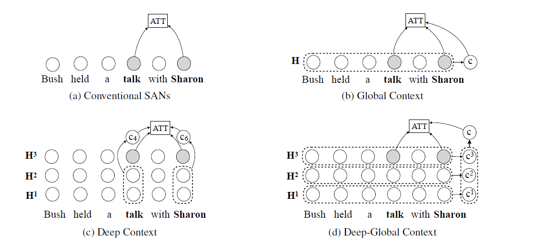
(b) Choices of Context Vectors
- Global Context : \(\mathbf{c}=\overline{\mathbf{H}} \quad \in \mathbb{R}^{d}\)
- Deep Context : \(\mathbf{C}=\left[\mathbf{H}^{1}, \ldots, \mathbf{H}^{l-1}\right] \quad \in \mathbb{R}^{n \times(l-1) d}\)
- Deep-Global Context : \(\mathbf{c}=\left[\mathbf{c}^{1}, \ldots, \mathbf{c}^{l}\right] \quad \in \mathbb{R}^{l d}\)
아래 그림으로 쉽게 이해 가능!