(PRML) Ch9.Mixture Models and EM

( Skip the basic parts + not important contents )

9. Mixture Models and EM

Begin mixture of distributions, by considering the problem of

“finding clusters” in a set of data points

• non-probabilistic ) K-means

• probabilistic ) EM algorithm

  ( = finding MLE in “latent variable models” )

K-means corresponds to a particular non-probabilistic limit of EM, applied to mixture of Gaussian!

9-1. K-means Clustering

substitute with my PPT

( download PPT here : Download )

loss function : \(J=\sum_{n=1}^{N} \sum_{k=1}^{K} r_{n k}\left\|\mathbf{x}_{n}-\boldsymbol{\mu}_{k}\right\|^{2}\)

where \(r_{n k}=\left\{\begin{array}{ll} 1 & \text { if } k=\arg \min _{j}\left\|\mathbf{x}_{n}-\boldsymbol{\mu}_{j}\right\|^{2} \\ 0 & \text { otherwise. } \end{array}\right.\).

solution : \(\boldsymbol{\mu}_{k}=\frac{\sum_{n} r_{n k} \mathbf{x}_{n}}{\sum_{n} r_{n k}}\)

9-2. Mixtures of Gaussian

Gaussian mixtures, in terms of DISCRETE LATENT variable

\(p(\mathbf{x})=\sum_{k=1}^{K} \pi_{k} \mathcal{N}\left(\mathbf{x} \mid \boldsymbol{\mu}_{k}, \mathbf{\Sigma}_{k}\right)\).

• \(\pi_{k}=p\left(z_{k}=1\right)\).
• \(0 \leqslant \pi_{k} \leqslant 1\).
• \(\sum_{k=1}^{K} \pi_{k}=1\).

\(p(\mathbf{x})=\sum_{\mathbf{z}} p(\mathbf{z}) p(\mathbf{x} \mid \mathbf{z})=\sum_{k=1}^{K} \pi_{k} \mathcal{N}\left(\mathbf{x} \mid \boldsymbol{\mu}_{k}, \mathbf{\Sigma}_{k}\right)\).

• \(p(\mathbf{z})=\prod_{k=1}^{K} \pi_{k}^{z_{k}}\).
• \(p(\mathbf{x} \mid \mathbf{z})=\prod_{k=1}^{K} \mathcal{N}\left(\mathbf{x} \mid \boldsymbol{\mu}_{k}, \mathbf{\Sigma}_{k}\right)^{z_{k}}\).
  • \(p\left(\mathrm{x} \mid z_{k}=1\right)=\mathcal{N}\left(\mathrm{x} \mid \mu_{k}, \Sigma_{k}\right)\).

We are able to work with joint pdf \(p(x,z)\), instead of \(p(x)\)

\(\rightarrow\) will lead to simplification, through “EM algorithm”

Responsibility

• conditional probability of \(z\), given \(x\)
• \(\begin{aligned} \gamma\left(z_{k}\right) \equiv p\left(z_{k}=1 \mid \mathrm{x}\right) &=\frac{p\left(z_{k}=1\right) p\left(\mathrm{x} \mid z_{k}=1\right)}{\sum_{j=1}^{K} p\left(z_{j}=1\right) p\left(\mathrm{x} \mid z_{j}=1\right)} \\ &=\frac{\pi_{k} \mathcal{N}\left(\mathrm{x} \mid \mu_{k}, \Sigma_{k}\right)}{\sum_{j=1}^{K} \pi_{j} \mathcal{N}\left(\mathrm{x} \mid \mu_{j}, \Sigma_{j}\right)} \end{aligned}\).

Interpretation

• \(\pi_k\) : prior probability of \(z_k=1\)
• \(\gamma\left(z_{k}\right)\) : posterior probability, once we have observed \(x\)

9-2-1. Maximum LIkelihood

observed data \(\mathbf{X}\): \(\left\{\mathrm{x}_{1}, \ldots, \mathrm{x}_{N}\right\}\), with size \(N \times D\)

latent variable : \(\mathbf{Z}\) : \(N \times K\) matrix

log likelihood : \(\ln p(\mathbf{X} \mid \pi, \boldsymbol{\mu}, \mathbf{\Sigma})=\sum_{n=1}^{N} \ln \left\{\sum_{k=1}^{K} \pi_{k} \mathcal{N}\left(\mathbf{x}_{n} \mid \boldsymbol{\mu}_{k}, \mathbf{\Sigma}_{k}\right)\right\}\).

problem with MLE : presence of singularities

ex) one of the data is \(\mu_{j}=\mathrm{x}_{n}\).

• \(\mathcal{N}\left(\mathbf{x}_{n} \mid \mathbf{x}_{n}, \sigma_{j}^{2} \mathbf{I}\right)=\frac{1}{(2 \pi)^{1 / 2}} \frac{1}{\sigma_{j}}\).
• as \(\sigma_{j} \rightarrow 0,\) log likelihood function will go to infinity

This will not happen, if we adopt “Bayesian Approach”!

9-2-2. EM for Gaussian Mixtures

will deal with…

• general treatment of EM

• how EM can be generalized to obtain VI framework

  ( VI = Variational Inference )

will take derivative of

\(\ln p(\mathbf{X} \mid \pi, \boldsymbol{\mu}, \mathbf{\Sigma})=\sum_{n=1}^{N} \ln \left\{\sum_{k=1}^{K} \pi_{k} \mathcal{N}\left(\mathbf{x}_{n} \mid \boldsymbol{\mu}_{k}, \mathbf{\Sigma}_{k}\right)\right\}\).

with

• 1) \(\mu_k\)
• 2) \(\sigma_k\)
• 3) \(\pi_k\)

(1) \(\mu_{k}=\frac{1}{N_{k}} \sum_{n=1}^{N} \gamma\left(z_{n k}\right) \mathrm{x}_{n}\)

\[0=-\sum_{n=1}^{N} \underbrace{\frac{\pi_{k} \mathcal{N}\left(\mathrm{x}_{n} \mid \mu_{k}, \Sigma_{k}\right)}{\sum_{j} \pi_{j} \mathcal{N}\left(\mathrm{x}_{n} \mid \mu_{j}, \Sigma_{j}\right)}}_{\gamma\left(z_{n k}\right)} \Sigma_{k}\left(\mathrm{x}_{n}-\mu_{k}\right)\]

• responsibilities \(\gamma(z_{nk})\) will appear!

• if we multiply \(\Sigma_k^{-1}\) on both sides…

\[\mu_{k}=\frac{1}{N_{k}} \sum_{n=1}^{N} \gamma\left(z_{n k}\right) \mathrm{x}_{n}\]

• where \(N_{k}=\sum_{n=1}^{N} \gamma\left(z_{n k}\right)\).

Interpretation

• \(N_k\) effective number of points assigned to cluster \(k\)

• \(\mu_k\) is obtained by taking “WEIGHTED mean” of all points,

  where each weight is posterior probability(responsibility) \(\gamma(z_{nk})\)

(2) \(\Sigma_{k}=\frac{1}{N_{k}} \sum_{n=1}^{N} \gamma\left(z_{n k}\right)\left(\mathrm{x}_{n}-\mu_{k}\right)\left(\mathrm{x}_{n}-\mu_{k}\right)^{\mathrm{T}}\)

• responsibilities \(\gamma(z_{nk})\) will appear!
• denominator : \(N_k\) ( effective number )

(3) \(\pi_{k}=\frac{N_{k}}{N}\)

constraint : \(\sum_{k=1}^{K} \pi_{k}=1\)

\[\ln p(\mathbf{X} \mid \pi, \mu, \Sigma)+\lambda\left(\sum_{k=1}^{K} \pi_{k}-1\right)\] \[0=\sum_{n=1}^{N} \frac{\mathcal{N}\left(x_{n} \mid \mu_{k}, \Sigma_{k}\right)}{\sum_{j} \pi_{j} \mathcal{N}\left(x_{n} \mid \mu_{j}, \Sigma_{j}\right)}+\lambda\]

• responsibilities \(\gamma(z_{nk})\) will appear!
• multiply both sides by \(\pi_k\) and sum over \(k\)

Then, \(\lambda=-N\) and thus \(\pi_{k}=\frac{N_{k}}{N}\)

Interpretation

• mixing coefficient for the \(k^{th}\) component is given by the average responsibilites

(4) Summary

Summary : all those (1)~(3) is NOT A CLOSED FORM solution

( \(\because\) responsibilities depend on those parameters! )

Therefore, suggest a “SIMPLE ITERATIVE SCHEME” = EM ALgorithm

• step 1) choose initial values for (1),(2),(3)
• step 2) alternate between the 2 steps
  • E step (Expectation step) : use current values of (1)(2)(3) to evaluate posterior)
  • M step (Maximization step) : re-estimate the (1)(2)(3)

Algorithm Summary

Goal : maximize the likelihood

1. Initialize the means \(\mu_{k}\), covariances \(\Sigma_{k}\) and mixing coefficients \(\pi_{k},\), and evaluate the initial value of the log likelihood.
   

2. E step. Evaluate the responsibilities using the current parameter values \(\gamma\left(z_{n k}\right)=\frac{\pi_{k} \mathcal{N}\left(\mathbf{x}_{n} \mid \boldsymbol{\mu}_{k}, \mathbf{\Sigma}_{k}\right)}{\sum_{j=1}^{K} \pi_{j} \mathcal{N}\left(\mathbf{x}_{n} \mid \boldsymbol{\mu}_{j}, \mathbf{\Sigma}_{j}\right)}\).
   

3. M step. Re-estimate the parameters using the current responsibilities

   \(\begin{aligned} \boldsymbol{\mu}_{k}^{\text {new }} &=\frac{1}{N_{k}} \sum_{n=1}^{N} \gamma\left(z_{n k}\right) \mathbf{x}_{n} \\ \boldsymbol{\Sigma}_{k}^{\text {new }} &=\frac{1}{N_{k}} \sum_{n=1}^{N} \gamma\left(z_{n k}\right)\left(\mathbf{x}_{n}-\boldsymbol{\mu}_{k}^{\text {new }}\right)\left(\mathbf{x}_{n}-\boldsymbol{\mu}_{k}^{\text {new }}\right)^{\mathrm{T}} \\ \pi_{k}^{\text {new }} &=\frac{N_{k}}{N} \end{aligned}\).

   where \(N_{k}=\sum_{n=1}^{N} \gamma\left(z_{n k}\right)\).

1. Evaluate the log likelihood

   \(\ln p(\mathbf{X} \mid \boldsymbol{\mu}, \boldsymbol{\Sigma}, \boldsymbol{\pi})=\sum_{n=1}^{N} \ln \left\{\sum_{k=1}^{K} \pi_{k} \mathcal{N}\left(\mathbf{x}_{n} \mid \boldsymbol{\mu}_{k}, \boldsymbol{\Sigma}_{k}\right)\right\}\).

1. return to Step 2, until convergence

9-3 An Alternative View of EM

Goal of EM : find ML solutions, for models “having LATENT VARIABLES”

ex) discrete r.v

\(\ln p(\mathbf{X} \mid \boldsymbol{\theta})=\ln \left\{\sum_{\mathbf{Z}} p(\mathbf{X}, \mathbf{Z} \mid \boldsymbol{\theta})\right\}\).

• (also apply equally to continuous case )

• key : summation over the latent variables “appears INSIDE the logarithm”

  • \(p(\mathbf{X}, \mathbf{Z} \mid \boldsymbol{\theta})\) : belongs to exponential family
  • \(p(\mathbf{X} \mid \boldsymbol{\theta})\) : does not belongs to exponential family

Concept

• \(\{\mathrm{X}, \mathrm{Z}\}\) : complete data
• \(\{\mathrm{X}\}\) : incomplete data

Likelihood function for complete dataset :

• simply takes the form \(\ln p(\mathbf{X} \mid \boldsymbol{\theta})\), and we shall maximize this! straight forward :)

• but, in practice, WE ARE NOT GIVEN COMPLETE data!

  ( just the incomplete data \(\mathbf{X}\) )

  ( \(Z\) is given by our posterior, \(p(Z \mid X,\theta)\) )

• So, instead “we use the expected value” under posterior of latent variable! That is E-STEP

E step

• use the current params \(\theta^{\text {old }}\) to find the posterior of the latent variables ( = \(p\left(\mathbf{Z} \mid \mathbf{X}, \theta^{\text {old }}\right)\) )

• Then, use this posterior to find the expectation of complete-data log likelihood!

  \(\mathcal{Q}\left(\boldsymbol{\theta}, \boldsymbol{\theta}^{\mathrm{old}}\right)=\sum_{\mathbf{Z}} p\left(\mathbf{Z} \mid \mathbf{X}, \boldsymbol{\theta}^{\mathrm{old}}\right) \ln p(\mathbf{X}, \mathbf{Z} \mid \boldsymbol{\theta})\).

M step

• determine the revised params \(\theta^{\text{new}}\),

  by maximizing \(\boldsymbol{\theta}^{\text {new }}=\underset{\theta}{\arg \max } \mathcal{Q}\left(\boldsymbol{\theta}, \boldsymbol{\theta}^{\text {old }}\right)\).

General EM Algorithm

1. initialize \(\theta^{\text {old }}\)

2. E step : evaluate \(P(\mathbf{Z} \mid \mathbf{X},\theta^{\text{old}})\).

3. M step : Evaluate \(\theta^{\text{new}}\), given by

   • \(\boldsymbol{\theta}^{\text {new }}=\underset{\theta}{\arg \max } \mathcal{Q}\left(\boldsymbol{\theta}, \boldsymbol{\theta}^{\text {old }}\right)\).

     where \(\mathcal{Q}\left(\boldsymbol{\theta}, \boldsymbol{\theta}^{\mathrm{old}}\right)=\sum_{\mathbf{Z}} p\left(\mathbf{Z} \mid \mathbf{X}, \boldsymbol{\theta}^{\mathrm{old}}\right) \ln p(\mathbf{X}, \mathbf{Z} \mid \boldsymbol{\theta})\).

4. Check for convergence

   • if convergence is not satisfied,

     \(\theta^{\text {old }} \leftarrow \theta^{\text {new }}\) and return to step 2

EM algorithm can also be used to find MAP

• prior \(p(\theta)\) is defined

• E step : same as ML case

  M step : target to be maximized = \(\mathcal{Q}\left(\boldsymbol{\theta}, \boldsymbol{\theta}^{\mathrm{old}}\right) + \text{ln}p(\theta)\)

Summary :

EM can be used in two cases

• 1) maximize likelihood, when there are “(discrete) latent variables”
• 2) ( same ), when unobserved variables correspond to missing values in the dataset

9-3-1. Gaussian mixtures revisted

apply this latent variable view of EM , to “GMM”

likelihood for complete data :

• (original) \(p(\mathbf{X}, \mathbf{Z} \mid \boldsymbol{\mu}, \boldsymbol{\Sigma}, \boldsymbol{\pi})=\prod_{n=1}^{N} \prod_{k=1}^{K} \pi_{k}^{z_{n k}} \mathcal{N}\left(\mathbf{x}_{n} \mid \boldsymbol{\mu}_{k}, \boldsymbol{\Sigma}_{k}\right)^{z_{n k}}\).

• (log) \(\ln p(\mathbf{X}, \mathbf{Z} \mid \boldsymbol{\mu}, \boldsymbol{\Sigma}, \boldsymbol{\pi})=\sum_{n=1}^{N} \sum_{k=1}^{K} z_{n k}\left\{\ln \pi_{k}+\ln \mathcal{N}\left(\mathbf{x}_{n} \mid \boldsymbol{\mu}_{k}, \boldsymbol{\Sigma}_{k}\right)\right\}\).

  ( \(\leftrightarrow\) unlike \(\ln p(\mathbf{X} \mid \boldsymbol{\mu}, \boldsymbol{\Sigma}, \boldsymbol{\pi})=\sum_{n=1}^{N} \ln \left\{\sum_{k=1}^{K} \pi_{k} \mathcal{N}\left(\mathbf{x}_{n} \mid \boldsymbol{\mu}_{k}, \boldsymbol{\Sigma}_{k}\right)\right\}\), logarithm now acts DIRECTLY on the Gaussian distn)

• advantage : can be maximized in closed form! ( \(\pi_{k}=\frac{1}{N} \sum_{n=1}^{N} z_{n k}\) )

  ( but in practice, it is not complete data…. therefore we need to use “expected” value of \(Z\) )

(1) Posterior distribution of latent variable \(Z\) :

\(p(\mathbf{Z} \mid \mathbf{X}, \boldsymbol{\mu}, \boldsymbol{\Sigma}, \boldsymbol{\pi}) \propto \prod_{n=1}^{N} \prod_{k=1}^{K}\left[\pi_{k} \mathcal{N}\left(\mathbf{x}_{n} \mid \boldsymbol{\mu}_{k}, \boldsymbol{\Sigma}_{k}\right)\right]^{z_{n k}}\).

(2) find the mean of “posterior of \(Z\) “

\(\begin{aligned} \mathbb{E}\left[z_{n k}\right] &=\frac{\sum_{z_{n k}} z_{n k}\left[\pi_{k} \mathcal{N}\left(\mathbf{x}_{n} \mid \boldsymbol{\mu}_{k}, \mathbf{\Sigma}_{k}\right)\right]^{z_{n k}}}{\sum_{z_{n j}}\left[\pi_{j} \mathcal{N}\left(\mathbf{x}_{n} \mid \boldsymbol{\mu}_{j}, \mathbf{\Sigma}_{j}\right)\right]^{z_{n j}}} \\ &=\frac{\pi_{k} \mathcal{N}\left(\mathbf{x}_{n} \mid \boldsymbol{\mu}_{k}, \mathbf{\Sigma}_{k}\right)}{\sum_{j=1}^{K} \pi_{j} \mathcal{N}\left(\mathbf{x}_{n} \mid \boldsymbol{\mu}_{j}, \mathbf{\Sigma}_{j}\right)}=\gamma\left(z_{n k}\right) \end{aligned}\).

(3) use that expected value(=(2)) to find complete-data log likelihood

\[\mathbb{E}_{\mathbf{Z}}[\ln p(\mathbf{X}, \mathbf{Z} \mid \boldsymbol{\mu}, \boldsymbol{\Sigma}, \boldsymbol{\pi})]=\sum_{n=1}^{N} \sum_{k=1}^{K} \gamma\left(z_{n k}\right)\left\{\ln \pi_{k}+\ln \mathcal{N}\left(\mathbf{x}_{n} \mid \boldsymbol{\mu}_{k}, \mathbf{\Sigma}_{k}\right)\right\}\]

(Summary)

• 1) initialize values for \(\mu^{\text {old }}, \Sigma^{\text {old }}\) and \(\pi^{\text {old }}\)
• 2) [E step] evaluate the responsibilities ( \(\gamma\left(z_{n k}\right)\), \(\mathbb{E}\left[z_{n k}\right]\), expected value of posterior of \(Z\) )
• 3) [M-step] keep \(\gamma\left(z_{n k}\right)\) fixed, and maximize “complete-data log likelihood” w.r.t \(\mu_{k}, \Sigma_{k},\pi_{k}\)

9-3-2. Relation to K-means

covariance matrices of the mixture components = \(\epsilon \mathbf{I}\)

\[p\left(\mathbf{x} \mid \boldsymbol{\mu}_{k}, \mathbf{\Sigma}_{k}\right)=\frac{1}{(2 \pi \epsilon)^{1 / 2}} \exp \left\{-\frac{1}{2 \epsilon}\left\|\mathbf{x}-\boldsymbol{\mu}_{k}\right\|^{2}\right\}\]

• treat \(\epsilon\) as a fixed constant!

(1) Initialize parameters

(2) evaluate responsibilities

\(\gamma\left(z_{n k}\right)=\frac{\pi_{k} \exp \left\{-\left\|\mathbf{x}_{n}-\boldsymbol{\mu}_{k}\right\|^{2} / 2 \epsilon\right\}}{\sum_{j} \pi_{j} \exp \left\{-\left\|\mathbf{x}_{n}-\boldsymbol{\mu}_{j}\right\|^{2} / 2 \epsilon\right\}}\).

(3) as \(\epsilon \rightarrow 0\) ,

• \[\gamma\left(z_{n k}\right) \rightarrow r_{n k}\]

  where \(r_{n k}=\left\{\begin{array}{ll} 1 & \text { if } k=\arg \min _{j}\left\|\mathbf{x}_{n}-\boldsymbol{\mu}_{j}\right\|^{2} \\ 0 & \text { otherwise. } \end{array}\right.\).

in the limit \(\epsilon \rightarrow 0\) , the expected complete-data log likelihood :

\(\mathbb{E}_{\mathbf{Z}}[\ln p(\mathbf{X}, \mathbf{Z} \mid \boldsymbol{\mu}, \mathbf{\Sigma}, \boldsymbol{\pi})] \rightarrow-\frac{1}{2} \sum_{n=1}^{N} \sum_{k=1}^{K} r_{n k}\left\|\mathbf{x}_{n}-\boldsymbol{\mu}_{k}\right\|^{2}+\text { const. }\).

• becomes “hard assignments”

Summary : EM re-estimation will reduce to K-means result!

9-3-3. Mixture of Bernoulli distributions

discuss mixture of discrete binary variables, “Bernoulli distribution”

( = known as “latent class analysis” )

\(\rightarrow\) foundation for a consideration of HMM over discrete variables

(1) without Mixture

\(p(\mathbf{x} \mid \boldsymbol{\mu})=\prod_{i=1}^{D} \mu_{i}^{x_{i}}\left(1-\mu_{i}\right)^{\left(1-x_{i}\right)}\).

• \(\mathbb{E}[\mathrm{x}] =\mu\).

  \(\operatorname{cov}[\mathrm{x}] =\operatorname{diag}\left\{\mu_{i}\left(1-\mu_{i}\right)\right\}\).

(2) with Mixture + without Latent Variable

\(p(\mathbf{x} \mid \boldsymbol{\mu}, \boldsymbol{\pi})=\sum_{k=1}^{K} \pi_{k} p\left(\mathbf{x} \mid \boldsymbol{\mu}_{k}\right)\).

• mix \(K\) components

• where \(p\left(\mathrm{x} \mid \boldsymbol{\mu}_{k}\right)=\prod_{i=1}^{D} \mu_{k i}^{x_{i}}\left(1-\mu_{k i}\right)^{\left(1-x_{i}\right)}\)

• \(\mathbb{E}[\mathbf{x}] =\sum_{k=1}^{K} \pi_{k} \mu_{k}\).

  \(\operatorname{cov}[\mathbf{x}] =\sum_{k=1}^{K} \pi_{k}\left\{\boldsymbol{\Sigma}_{k}+\boldsymbol{\mu}_{k} \boldsymbol{\mu}_{k}^{\mathrm{T}}\right\}-\mathbb{E}[\mathbf{x}] \mathbb{E}[\mathbf{x}]^{\mathrm{T}}\).

  • where \(\mathbf{\Sigma}_k=\operatorname{diag}\left\{\mu_{k i}\left(1-\mu_{k i}\right)\right\} .\)

Log likelihood function : \(\ln p(\mathbf{X} \mid \mu, \pi)=\sum_{n=1}^{N} \ln \left\{\sum_{k=1}^{K} \pi_{k} p\left(\mathbf{x}_{n} \mid \boldsymbol{\mu}_{k}\right)\right\}\)

• summation “inside” the log :(

  \(\rightarrow\) no longer closed form …

• use “EM ALGORITHM”

(3) with Mixture + with Latent Variable

• introduce an explicit latent variable \(z\)
• (a) conditional distn of \(x\), given \(z\) : \(p(\mathbf{x} \mid \mathbf{z}, \boldsymbol{\mu})=\prod_{k=1}^{K} p\left(\mathbf{x} \mid \boldsymbol{\mu}_{k}\right)^{z_{k}}\)
• (b) prior : \(p(\mathbf{z} \mid \pi)=\prod_{k=1}^{K} \pi_{k}^{z_{k}}\)

product of (a) and (b) & marginalize over \(z\) : \(p(\mathbf{x} \mid \boldsymbol{\mu}, \boldsymbol{\pi})=\sum_{k=1}^{K} \pi_{k} p\left(\mathbf{x} \mid \boldsymbol{\mu}_{k}\right)\)

Use EM Algorithm

step 1) write down complete-data log likelihood :

• \(\begin{array}{l} \ln p(\mathbf{X}, \mathbf{Z} \mid \boldsymbol{\mu}, \boldsymbol{\pi})=\sum_{n=1}^{N} \sum_{k=1}^{K} z_{n k}\left\{\ln \pi_{k}\right. \left.\quad+\sum_{i=1}^{D}\left[x_{n i} \ln \mu_{k i}+\left(1-x_{n i}\right) \ln \left(1-\mu_{k i}\right)\right]\right\} \end{array}\).

• \(\begin{aligned} \mathbb{E}_{\mathbf{Z}}[\ln p(\mathbf{X}, \mathbf{Z} \mid \boldsymbol{\mu}, \boldsymbol{\pi})] &=\sum_{n=1}^{N} \sum_{k=1}^{K} \gamma\left(z_{n k}\right)\left\{\ln \pi_{k}\right. \left.+\sum_{i=1}^{D}\left[x_{n i} \ln \mu_{k i}+\left(1-x_{n i}\right) \ln \left(1-\mu_{k i}\right)\right]\right\} \end{aligned}\).

step 2) E-step: calculate responsibilities

• \(\begin{aligned} \gamma\left(z_{n k}\right)=\mathbb{E}\left[z_{n k}\right] &=\frac{\sum_{z_{n k}} z_{n k}\left[\pi_{k} p\left(\mathbf{x}_{n} \mid \boldsymbol{\mu}_{k}\right)\right]^{z_{n k}}}{\sum_{z_{n j}}\left[\pi_{j} p\left(\mathbf{x}_{n} \mid \boldsymbol{\mu}_{j}\right)\right]^{z_{n j}}} =\frac{\pi_{k} p\left(\mathbf{x}_{n} \mid \boldsymbol{\mu}_{k}\right)}{\sum_{j=1}^{K} \pi_{j} p\left(\mathbf{x}_{n} \mid \boldsymbol{\mu}_{j}\right)} \end{aligned}\).
• responsibilities enter only through 2 terms
  • \(N_{k} =\sum_{n=1}^{N} \gamma\left(z_{n k}\right)\).
  • \(\overline{\mathrm{x}}_{k} =\frac{1}{N_{k}} \sum_{n=1}^{N} \gamma\left(z_{n k}\right) \mathrm{x}_{n}\).

step 3) M-step : maximize the expected complete-log likelihood ( w.r.t \(\mu\) and \(\pi\) )

• \(\mu_{k}=\overline{\mathrm{x}}_{k}\).
• \(\pi_{k}=\frac{N_{k}}{N}\).

Conjugate prior

• Bernoulli - Beta
• Multinomial - Dirichlet

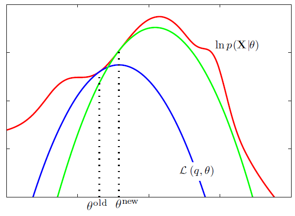
9-4. The EM Algorithm in General

EM : form the basis of Variational Inference framework

Goal : maximize \(p(\mathbf{X} \mid \boldsymbol{\theta})=\sum_{\mathbf{Z}} p(\mathbf{X}, \mathbf{Z} \mid \boldsymbol{\theta})\)

• optimization of \(p(\mathbf{X}\mid \theta)\) is difficult

• optimization of \(p(\mathbf{X},\mathbf{Z} \mid \theta)\) is easy!

  \(\rightarrow\) thus, introduce latent variable \(\mathbf{Z}\)

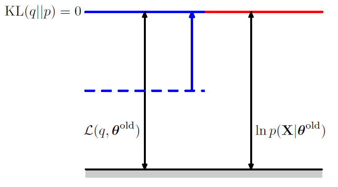
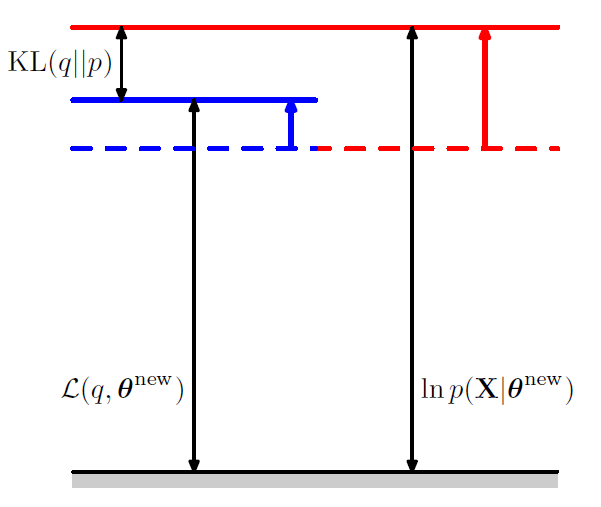
\(\ln p(\mathbf{X} \mid \boldsymbol{\theta})=\mathcal{L}(q, \boldsymbol{\theta})+\mathrm{KL}(q \| p)\).

• \(\mathcal{L}(q, \boldsymbol{\theta}) =\sum_{\mathbf{Z}} q(\mathbf{Z}) \ln \left\{\frac{p(\mathbf{X}, \mathbf{Z} \mid \boldsymbol{\theta})}{q(\mathbf{Z})}\right\}\). …. ELBO ( = Variational Free Energy )
• \(\mathrm{KL}(q \| p) =-\sum_{\mathbf{Z}} q(\mathbf{Z}) \ln \left\{\frac{p(\mathbf{Z} \mid \mathbf{X}, \boldsymbol{\theta})}{q(\mathbf{Z})}\right\}\).

[ E step ]

• maximize \(\mathcal{L}\left(q, \boldsymbol{\theta}^{\text {old }}\right)\) w.r.t \(q(\mathbf{Z})\), while holding \(\boldsymbol{\theta}^{\text {old }}\) fixed

• substitute \(q(\mathbf{Z})=p\left(\mathbf{Z} \mid \mathbf{X}, \boldsymbol{\theta}^{\text {old }}\right)\)

  then,

  \[\begin{aligned} \mathcal{L}(q, \boldsymbol{\theta}) &=\sum_{\mathbf{Z}} p\left(\mathbf{Z} \mid \mathbf{X}, \boldsymbol{\theta}^{\text {old }}\right) \ln p(\mathbf{X}, \mathbf{Z} \mid \boldsymbol{\theta})-\sum_{\mathbf{Z}} p\left(\mathbf{Z} \mid \mathbf{X}, \boldsymbol{\theta}^{\text {old }}\right) \ln p\left(\mathbf{Z} \mid \mathbf{X}, \boldsymbol{\theta}^{\text {old }}\right) \\ &=\mathcal{Q}\left(\boldsymbol{\theta}, \boldsymbol{\theta}^{\text {old }}\right)+\text { const } \end{aligned}\]

  • constant is just negative entropy of \(q\) distn

  • independent of \(\theta\)

  

[ M step ]

• maximize \(\mathcal{L}\left(q, \boldsymbol{\theta}^{\text { }}\right)\) w.r.t \(\theta\), while holding \(q(\mathbf{Z})\) fixed

  ( = expectation of the complete-data log likelihood is maximized )

  

Total Summary with one picture!