
[Deep Bayes] 01. Bayesian Framework
해당 내용은 https://deepbayes.ru/ (Deep Bayes 강의)를 듣고 정리한 내용이다.
1. Introduction
이번 포스트에서는, 앞으로 다루게 될 내용인 Bayesian Statistics의 기초가 되는 내용을 다룰 것이다. (1) Bayesian Framework가 무엇인지 확인하고 (Frequentist와 비교한 Bayesian의 특징), (2) Bayesian ML model들의 개요에 대해 설명한 뒤, (3) Conjugate Distribution에 대해서 알아 볼 것이다.
2. Bayesian Framework
우선 다들 어느 정도 Bayesian Statistics에 대해 알고 있다는 가정 하에 설명을 할 것이다. 그래도 가볍게 다시 한번 짚고 넘어가보자.
[ Bayes’ Theorem ]
Bayes’ Theorem에 따르면, 조건부 확률(conditional probability)은 다음과 같이 표현할 수 있다.
\[p(x\mid y) = \frac{p(x,y)}{p(y)}\]위 식에서 좌변을 ‘Conditional Probability‘이라고 하고, 우변의 분자는 ‘Joint Probability’, 우변의 분모는 (x에 대해 marginalize한) ‘Marginal Probability‘라고 한다.
그리고 우리는 Joint Distribution에 대해 다음과 같은 Product rule을 적용하여 표현할 수 있다.
\[p(x,y,z) = p(x \mid y,x) p(y\mid z)p(z)\]또한, Marginal Distribution을 다음과 같은 Sum rule을 적용하여 표현할 수 있다.
\[p(y) = \int p(x,y)dx\]이 두 rule을 적용하여, 우리는 Bayes Theorem을 다음과 같이 표현할 수 있다.
\[p(y\mid x) = \frac{p(x,y)}{p(x)} = \frac{p(x\mid y)p(y)}{p(x)} =\frac{p(x\mid y)p(y)}{\int p(x\mid y)p(y)dy}\]위 식에서, 우리는 좌변의 \(p(y\mid x)\) 를 Posterior라고 부르고, 우변의 분자 중 \(p(x\mid y)\)를 Likelihood, \(p(y)\)를 Prior, 분모 \(\int p(x\mid y)p(y)dy\) 를 Evidence라고 부른다. 자주 사용하게 될 표현이니 익숙해질 필요가 있다.
\[Posterior = \frac{Likelihood \times Prior}{Evidence}\][ Frequentist vs Bayesian ]
우선, 우리에겐 다음과 같은 문제 상황이 주어진다.
problem : 확률 분포 \(p(x\mid \theta)\) 로 부터 데이터 \(X = (x_1,x_2,...,x_n)\) 이 주어졌을 때, 모수 \(\theta\)를 예측하라!
이를 해결하기 위한 큰 두 가지 접근 법에는 (1) Frequentist Framework와 (2) Bayesian Framework가 있다.
(1) Frequentist Framework
많이 들 알겠지만, MLE (Maximum Likelihood Estimation)가 Frequentist Framework의 대표적인 방법이다. 이들은 다음과 같은 방법을 통해 모수를 추정한다.
\[\theta_{ML} = argmax\; p(X\mid \theta) = argmax\; \prod_{i=1}^{n}p(x_i\mid \theta) = argmax\; \sum_{i=1}^{n}logp(x_i,\theta)\](2) Bayesian Framework
우리가 앞으로 다루게 될 내용은 위와 다르게, 모수 \(\theta\)는 정해진 값이 아니라 어떠한 분포를 가진다는 가정 하에 다음과 같은 식을 통해 모수를 추정할 것이다.
\[p(\theta \mid X) = \frac{ \prod_{i=1}^{n}p(x_i\mid \theta)p(\theta)}{\int \prod_{i=1}^{n}p(x_i\mid \theta)p(\theta)d\theta}\](3) Advantages of Bayesian Framework
Bayesian Framework를 사용하면 좋은 점들은 다음과 같다.
- 1 ) Prior Knowledge를 사용할 수 있다 ( \(p(\theta)\) )
- 2 ) 우리가 추정한 모수 \(\theta\)에 대해 uncertainty도 파악할 수 있다.
여기서 알야할 것은, Bayesian Framework와 Frequentist Framework는 서로 상충되는 개념이 아니라는 것이다. 그저 문제 해결을 위해 바라보는 관점이 다를 뿐이라는 점이다.
3. Probabilistic ML Model
우선, 개념부터 간단히 정리해보자
- \(x\) : 관측된 값들 ( set of observed variables )
- \(y\) : 숨겨진/잠재된 값들 ( set of hidden / latent variables )
- \(\theta\) : 추정하고 싶은 모델의 모수 ( model parameters )
Probabilistic ML Model에는 다음과 같이 크게 두 가지의 모델이 존재한다.
- 1 ) Discriminative probabilistic ML model
- 2 ) Generative probabilistic ML model
(1) Discriminative probabilistic ML model
model : \(p(y,\theta \mid x)\)
목적 : 데이터(x)가 주어 졌을 때, 결과(y) 예측하기
가정 : (주로) 모수 \(\theta\)가 \(x\)에 의존(depend)하지 않는다고 가정한다
예시 : 흔히 ML에서 많이 사용하는 모델들이 여기에 속한다.
- 분류(Classification), 회귀(Regression) 모델
- 기계 번역 (Machine Translation)
(2) Generative probabilistic ML model
model : \(p(x,y,\theta) = p(x,y \mid \theta) p(\theta)\)
목적 : 새로운 object를 생성! ( pairs \((x,y)\) )
예시 : 최근에 화두가 되고 있는 GAN(Generative Adversarial Network)가 이것의 대표적인 예이다.
Training & Testing Bayesian ML models
( Discriminative probabilistic ML model에 대해서 다룰 것이다 )
그렇다면 어떻게 위 모델을 학습시킬 것인가?
이 모델의 Training Stage와 Testing Stage에 대해 알아보자.
Training Stage : \(\theta\)에 대해 Bayesian Inference를 한다.
\[p(\theta \mid X_{tr}, Y_{tr}) = \frac{p(Y_{tr}\mid X_{tr},\theta)p(\theta)}{\int p(Y_{tr}\mid X_{tr},\theta)p(\theta)d\theta}\]이렇게 해서 나오게 된 결과들을 종합(ensemble)한다. ( 하나의 추정된 \(\theta_{ML}\) 를 사용하는 것 보다, 여러 알고리즘을 사용하여 추정된 여러 \(\theta\)를 ensemble하는 것이 주로 더 좋은 결과를 보인다 )
Testing Stage : Training Stage를 통해 추정해낸 \(\theta\)를 사용하여, 새로운 데이터 \(x\)에 대한 예측 값을 낸다.
\[p(y \mid x, X_{tr}, Y_{tr}) = \int p(y \mid x,\theta)\; p(\theta \mid X_{tr}, Y_{tr})d\theta\]위의 두 수식 대로 풀어서 \(\theta\)를 구하는 것을 Full Bayesian Inference라고 한다.
4. Conjugate Distribution
위에서 언급한 두 식 \(p(\theta \mid X_{tr}, Y_{tr}) = \frac{p(Y_{tr}\mid X_{tr},\theta)p(\theta)}{\int p(Y_{tr}\mid X_{tr},\theta)p(\theta)d\theta}\) 의 (우변의) 분모는 그 형태에 따라 다루기 쉬울 수도 있지만, 복잡한 모델의 경우 다루기 어려울 수 있다 (intractable).
위 식을 개념적으로 나타내면 \(Posterior = \frac{Likelihood \times Prior}{Evidence}\)과 같고, 즉 여기서 Evidence를 구하기 어려울 수 있다는 것이다. 하지만, 특정한 경우에 우리는 이 문제를 쉽게 풀 수 있다. 특정 Likelihood에 대해서, Prior를 특정 분포로 사용했을 때, Posterior도 이와 동일한 분포를 띄는 경우이다. 이런 경우를 우리는 Conjugate하다고 표현한다.
그럴 경우, 우리는 intractable한 분모 부분 (evidence)를 신경 쓰지 않고 분자 부분인 Likelihood x Prior만 신경 쓰면 된다.
\[p(y\mid x) = \frac{p(x\mid y)p(y)}{\int p(x\mid y)p(y) dy} \propto p(x\mid y)p(y)\]Example
Conjugate한 케이스의 예시 중 하나로, likelihood가 Bernoulli Distribution이고 prior가 Beta Distribution일 경우 이 둘은 서로 conjugate한다. 다음 식을 통해 확인해보자
Likelihood : \(p(x\mid \theta) = \theta^{x} (1-\theta)^{1-x}\)
Prior : \(p(\theta) = \frac{1}{B(a,b)} \theta^{a-1}(1-\theta)^{b-1}\)
( 여기서 \(B(a,b) = \frac{\Gamma(a + b)}{\Gamma(a) + \Gamma(b)} 이다)\)
편의상, \(\theta\)와 상관 없는 부분들을 제외하고 prior를 다음과 같이 표현하자.
\[p(\theta) = C\;\theta^{\alpha}(1-\theta)^{\beta}\]그러면, 우리는 다음과 같은 posterior를 얻을 수 있다.
\[\begin{align*} p(\theta \mid x) &= C'\;p(x\mid \theta)p(\theta) \\ &= C'\; \theta^{x}(1-\theta)^{1-x}\;\frac{1}{B(a,b)} \theta^{a-1}(1-\theta)^{b-1}\\ &= C''\; \theta^{\alpha '}(1-\theta)^{\beta '} \end{align*}\]위에서 보다시피, prior \(p(\theta) = C\;\theta^{\alpha}(1-\theta)^{\beta}\)와 posterior \(p(\theta \mid x) = C''\; \theta^{\alpha '}(1-\theta)^{\beta '}\)는 서로 동일한 형태를 띈다. 따라서 이 경우, 이 둘은 서로 conjugate하다.
이 경우 외에도, 다양한 Conjugate Distribution이 있다.
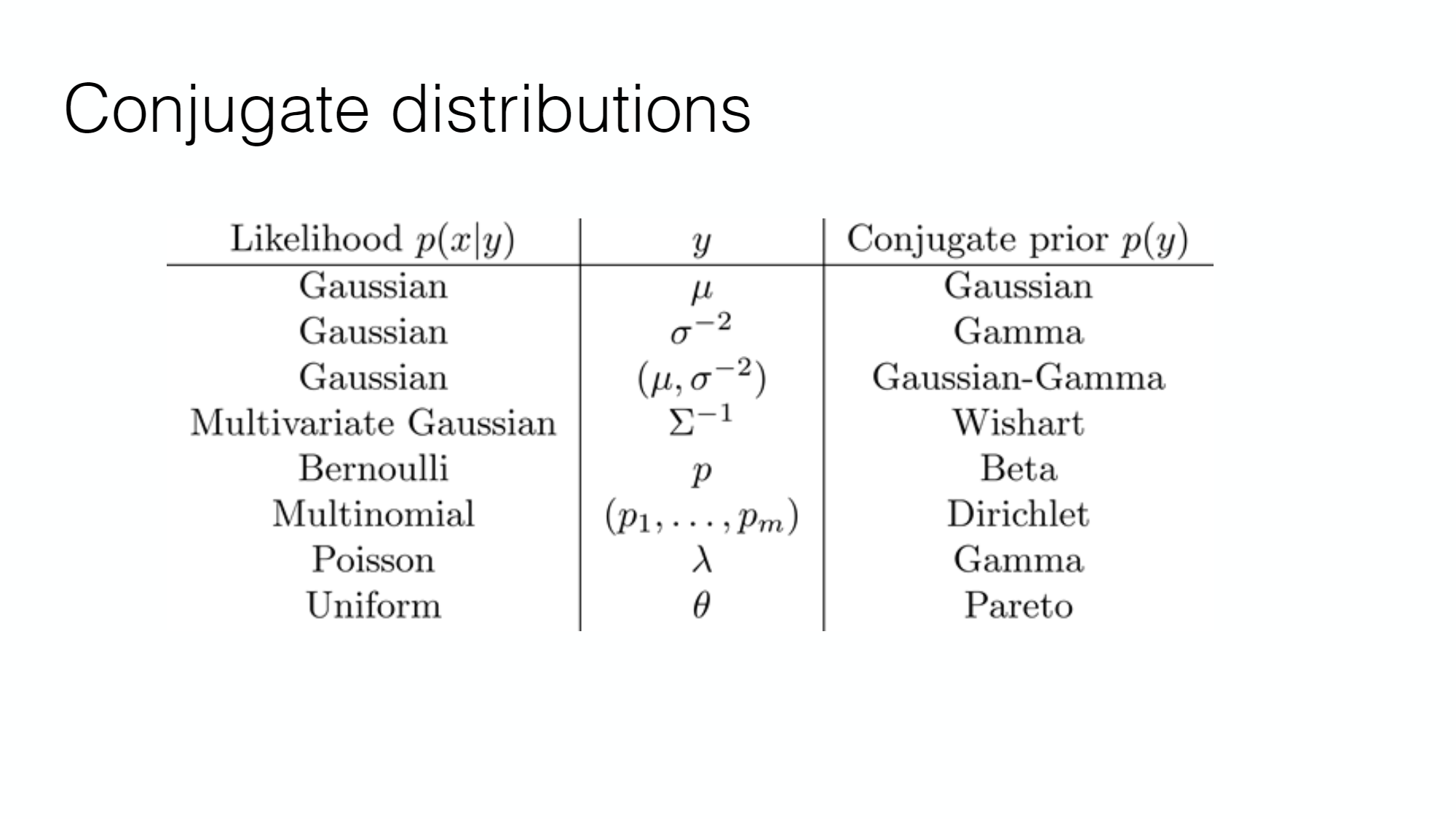
하지만, 위와 같이 Conjugate 쌍을 이루지 않는 경우가 많다.
이럴 경우에는 어떻게 해결할지 다음 포스트에서 알아보자.