
4. Variational Inference
( Assume that we all know Jensen’s Inequality, KL-Divergence, Variational Transform - look at the previous three posts )
(1) Applying Convex Duality to Probability Function
PDF is also a ‘function’. So we can also apply the Convex Duality to pdf.
Example
Let’s take an example
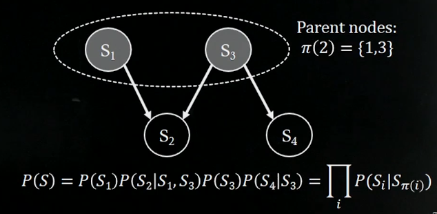
We can express \(P(S)\) like the joint pdf above. So, how can we express this more easily?
Do you remember \(f(x) = min_{\lambda}{\lambda^T x-f^{*}(\lambda)}\) ?
If we apply the same method to the problem above, we could express it like the below!
( by introducing a “more simple function \(P^U\)” and a “variational parameter \(\lambda^U\) )
\(P(S) = \prod_{i}P(S_i \mid S_{\pi(i)}) = min_\lambda \prod_{i} P^U(S_i\mid S_{\pi(i)},\lambda^U_i)\)
\(P(S) = \prod_{i}P(S_i \mid S_{\pi(i)}) \leq \prod_{i} P^U(S_i\mid S_{\pi(i)},\lambda^U_i)\)
What we can know from this expression is that “We can express pdf with a more simpler function”. But we get a new variational parameter to optimize.
(2) Variables of E & H
E stands for “Evidence”, which is the observed. And H stands for “Hypothesis”, which is the estimated.
How do we get \(P(H\mid E)\)?
With Bayes’ Theorem, \(P(H\mid E) = P(H,E) / P(E)\)
To solve this, we have to find the joind pdf and the \(P(E)\). And we are going to use Variational Inference to find out \(P(E)\)!
(3) MFVI (Mean Field Variational Inference)
By using Jensen’s Inequality and KL-Divergence, we can find out ELBO (evidence lower bound).
\(L(\lambda,\theta) = \sum_H Q(H\mid E,\lambda)\; lnP(H,E\mid \theta) - Q(H\mid E,\lambda)\; lnQ(H\mid E,\lambda)\)
And with EM algorithm…
- E step : \(\lambda^{t+1} = \underset{\lambda}{argmax}L(\lambda^{t},\theta^{t})\)
- M step : \(\theta^{t+1} = \underset{\theta}{argmax}L(\lambda^{t+1},\theta^{t})\)
So, how should we make \(Q\)? ( = how can we make \(Q(H\mid E,\lambda)=P(H\mid E,\theta)\)? )
We’ll use mean-field approximation to set Q. That is, we will use “multiple” hidden variables, assuming that they are independent. So we will make \(Q\) function like below :
\(Q(H) = \prod_{i\leq \mid H\mid} q_i(H_i,\lambda_i)\)
This assumption is quite strong, but makes our problem more simple and easier to handle.
When we make the assumption like above and set \(Q\) function like that, we call this MFVI(Mean Field Variational Inference).
(4) How to solve?
With the Mean Field assumption , we can express \(L(\lambda,\theta)\) like below.
\[\begin{align*} L(\lambda,\theta) &=\sum_H Q(H\mid E,\lambda)lnP(H,E\mid \theta) - Q(H\mid E,\lambda)lnQ(H\mid E,\lambda)\\ &=\sum_H\{ \prod_{i\leq \mid H\mid}q_i(H_i\mid E,\lambda_i)lnP(H,E\mid \theta) - \prod_{i\leq \mid H\mid}q_i(H_i\mid E,\lambda_i)ln\prod_{k\leq \mid H \mid}q_k(H_i \mid E, \lambda_i)\} \\ &=\sum_H\{ \prod_{i\leq \mid H\mid}q_i(H_i\mid E,\lambda_i)lnP(H,E\mid \theta) - \prod_{i\leq \mid H\mid}q_i(H_i\mid E,\lambda_i)\sum_{k\leq \mid H \mid} lnq_k(H_k\mid E, \lambda_k)\} \\ \end{align*}\]We had decomposed \(Q\) into small \(q_i\) , and $\lambda$ into \(\lambda_i\).
If we express the expression with respect to \(\lambda_j\),
.png)
( all the parameters except \(\lambda_j\) ( which are \(\lambda_{-j}\) & \(\theta\) ) are regarded as constant. )
We got an equation like the below.
\(\begin{align*} L(\lambda_j) &= \sum_{H_j}q_j(H_j\mid E, \lambda_j) \sum_{H_{-j}}\prod_{i\leq \mid H \mid, i \neq j}q_i(H_i\mid E,\lambda_i) lnP(H,E\mid \theta) \\&- \sum_{H_j}q_j(H_j\mid E,\lambda_j)lnq_j(H_j\mid E,\lambda_j)+C \end{align*}\)
So how do we make this equation more simple?
We change the part \(\sum_{H_{-j}}\prod_{i\leq \mid H \mid, i \neq j}q_i(H_i\mid E,\lambda_i) lnP(H,E\mid \theta)\) into a new P function, \(ln\widetilde{P}(H,E\mid \theta)\)
\(ln\widetilde{P}(H,E\mid \theta)\) = \(\sum_{H_{-j}}\prod_{i\leq \mid H \mid, i \neq j}q_i(H_i\mid E,\lambda_i) lnP(H,E\mid \theta) = E_{q_{i\neq j}}[lnq_i(H_i\mid E,\lambda_i)]+C\)
Then we can get \(L(\lambda_i)\) like below
\(L(\lambda_i) = \sum_{H_j}q_j(H_j\mid E, \lambda_j) ln\widetilde{P}(H,E\mid \theta)\) - \(\sum_{H_j}q_j(H_j\mid E,\lambda_j)lnq_j(H_j\mid E,\lambda_j)+C\)
Until now, we have decomposed \(Q\) into multiple \(q_i\) s, and made a big problem into solving small optimization problems related to every \(q_i\)s.
What do we have to solve?
- BEFORE : \(Q(H\mid E,\lambda) = P(H \mid E,\theta)\)
- AFTER : \(lnq_i^{*}(H_i \mid E, \lambda_i)\) = \(ln\widetilde{P}(H,E\mid \theta)\) = \(E_{q_{i\neq j}}[lnP(H,E\mid \theta)]+C\)