2. EM Algorithm (1)

There are two important concepts that you have to know, before knowing about EM Algorithm. They are 1. Jensen’s inequality & 2. KL-divergence.

(1) Jensen’s inequality & KL-divergence

[ Jensen’s inequality ]

convex / concave
relates the value of a convex/convex function of an integral to the integral of the convex/concave function
in the case of concave function..

If $f(\alpha a + (1-\alpha)b) \geq \alpha f(a) + (1-\alpha)f(b)$

Then Jensen’s inequality is $f(E_{p(t)}t)\geq E_{p(t)}f(t)$

( a, b is a any two data point. alpha is a weight between 0 and 1 )

https://encrypted-tbn0.gstatic.com/

[ KL-divergence ]

KL-divergence( Kullback–Leibler divergence), which is also called relative entropy, is a measure of how one probability distribution is different from another probability distribution.

For a discrete probability distribution, the KL-divergence of Q from P is

and for a continuous case, it is

https://cs-cheatsheet.readthedocs.io/en/latest/_images/kl_divergence.png

The three properties of KL-divergence are

$KL(p \mid q)$ is not always same with $KL(q \mid p)$
\[KL(p \mid p) = 0\]
$$KL(p \mid q)$ is always more or equal to 0

(2) EM algorithm

( EM : Expectation-Maximization )

EM algorithm is one way of finding MLE in a probabilistic model which has latent variable. Before talking about this algorithm in detail, I’ll start with an example.

example )

Remember soft clustering using GMM in the previous post? ( https://seunghan96.github.io/em%20algorithm/8.-em-Latent_Variable_Models/)

We had three mixture of Gaussian distribution ( 3 clusters ). We wanted to find the density of each data point ( $= p(X \mid \theta)$ ) I told you that I will find this solution with EM algorithm, and I’m going to talk about that now. ( since now you know what Jensen’s Inequality & KL-divergence are ).

We take logarithm of the likelihood ( $= p(X \mid \theta)$ ) for easier calculation. Then using Jensen’s Inequality, we can make the expression like below.

$\begin{align*} logp(X|\theta) &= \sum_{i=1}^{N}logp(x_i|\theta) \\ &= \sum_{i=1}^{N}log \sum_{c=1}^{3}\frac{q(t_i=c)}{q(t_i=c)}p(x_i,t_i=c|\theta)\\ &\geq \sum_{i=1}^{N}\sum_{c=1}^{3}q(t_i=c)log\frac{p(x_i,t_i=c|\theta)}{q(t_i=c)}\\ &=L(\theta,q) \end{align*}$

[ Interpretation ]

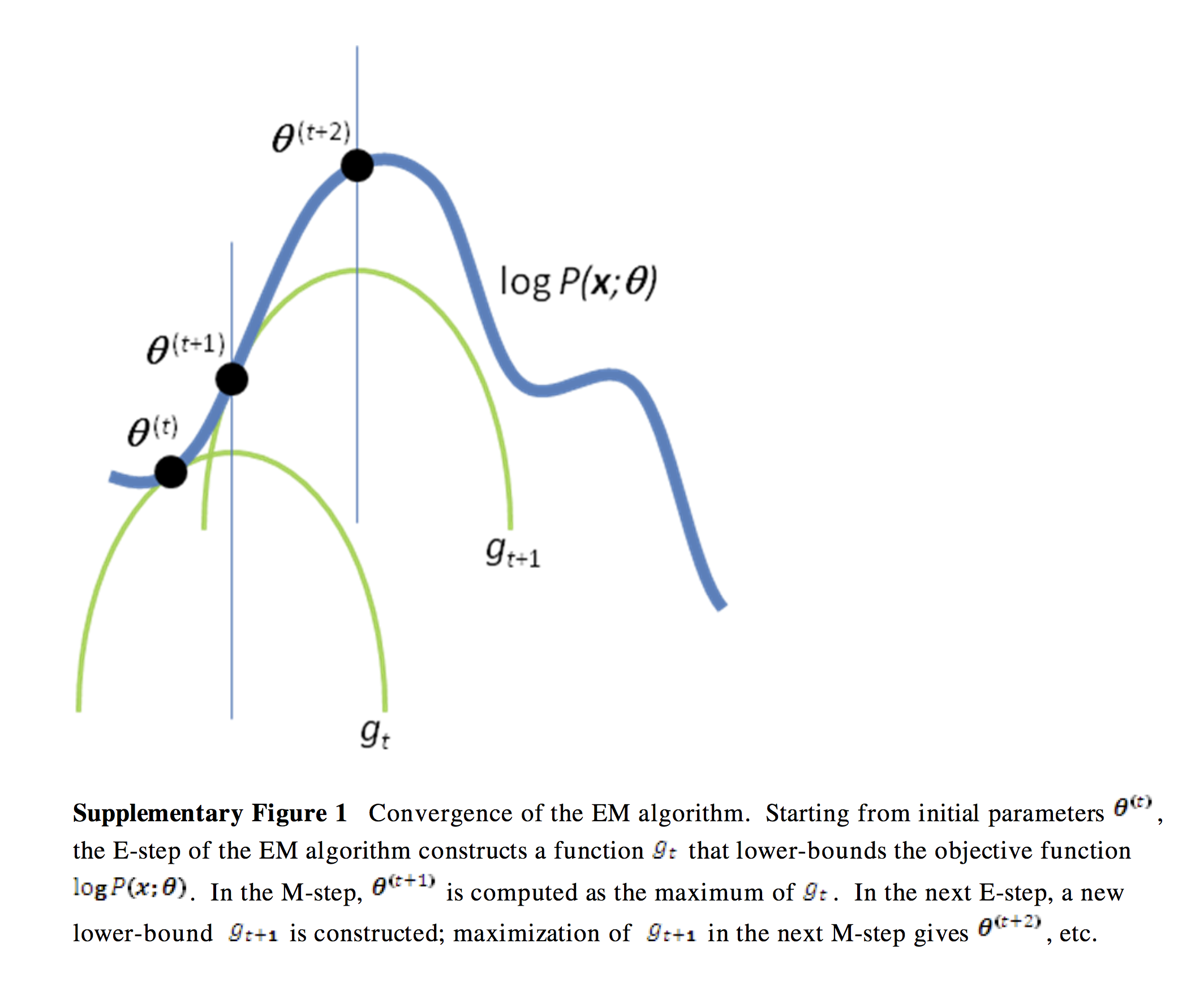
We built a lower bound by using Jensen’s Inequality, which is expressed as $L(\theta,q)$. Now, we are going to maximize this. Instead of directly maximizing the likelihood, we can maximize the lower bound instead to find the value of $log p(X \mid \theta)$. But we will not only use one lower bound. Instead, we can use a family of lower bounds, and choose the one that suits best at each iteration. Look at the picture below, and you will understand what I mean.

https://people.duke.edu/~ccc14/sta-663/

The best lower bound among the lower bound family is chosen with the following expression. ( The best possible bound is when $log\;p(X\mid \theta)$ = $L(\theta,q)$ )

$logp(X|\theta)\geq L(\theta,q) \;\; for \; any \; q$

$q^{k+1} = \underset{q}{argmax}L(\theta^k,q)$

That’s all! Quite Simple!

In short, all we have to do is maximizing the lower bound. So how do we maximize it? We do it iteratively (E-step & M-step). First, we fix $\theta$, and maximize the lower bound with respect to $q$. Then, we fix $q$, and do the same thing with respect to $\theta$. No you have seen how EM algorithm is applied to GMM.

Algorithm Summary

E-step : fix $\theta$, maximize the lower bound with respect to q

$q^{k+1} = \underset{q}{argmax}L(\theta^k,q)$
M-step : fix $q$, maximize the lower bound with respect to theta

$\theta^{k+1} = \underset{\theta}{argmax}L(\theta,q^{k+1})$

In the next post, I’ll tell you more about EM algorithm in detail.

Twitter Facebook LinkedIn

10.(EM algorithm) EM algorithm (1)

Seunghan Lee