Accurate predictions on small data with a tabular foundation model

Accurate predictions on small data with a tabular foundation model

Contents

1. Abstract
2. Introduction
3. An architecture designed for tables
4. Synthetic data based on causal models
5. Qualitative analysis
6. Quantitative analysis
7. Foundation model with interpretability
8. Conclusion

Abstract

Tabular Prior-data Fitted Network (TabPFN)

• Tabular foundation model
• Outperforms all previous methods on datasets with up to 10,000 samples
• Substantially less training time.

1. Introduction

(1) TabPFN

• Foundation model for small to medium-sized tabular data
• Dominant performance for datasets with up to 10,000 samples and 500 features
• Single forward pass
• Generate a large corpus of synthetic tabular datasets & Pretrain a transformer

(2) Principled ICL

ICL

• Shown that transformers can learn simple algorithms such as logistic regression through ICL

Prior-data Fitted Networks (PFNs)

• Shown that even complex algorithms (e.g., Gaussian Processes and Bayesian Neural Networks) can be approximated with ICL

TabPFN-v2

• Build on a preliminary version of TabPFN
• vs. TabPFN
  • Scales to 50 x larger datasets
  • Supports regression tasks, categorical data and missing values
  • Robust to unimportant features and outliers

Standard setting vs. ICL

• Standard setting
  • (Train) Per dataset
  • (Inference) Applied to test samples
• ICL
  • (Train) Across datasets
  • (Inference) Applied to entire datasets (rather than individual samples)

Pretraining & Inference of TabPFN

• [Pretraining] Pre-trained on millions of synthetic datasets

• [Inference] Unseen dataset with..

  • (1) Training (X,y)
  • (2) Test (X)

  \(\rightarrow\) Predict Test (y)

(3) Overview

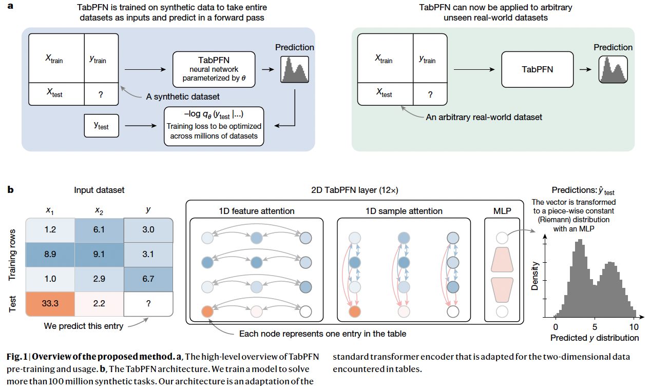
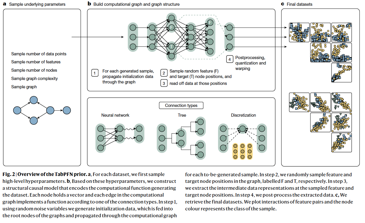
a) Data generation

• Pretraining dataset = Synthetic dataset = Prior
• Varying relationships between features and targets
• Millions of datasets from the generative process

b) Pre-training

• Pretrain a transformer model
• Predict the masked targets of all synthetic datasets
• Done only once during model development

c) Real-world prediction

• Can be used to predict any arbitrary unseen real-world datasets
• Training samples are provided as context (feat. ICL)

2. An architecture designed for tables

Although transformer-based models can be applied to tabular data…

TabPFN addresses TWO key limitations

• (1) Transformers treat the input data as a single sequence, not using the tabular structure
• (2) Transformer-based ICL algorithms receive train and test data in a single pass and thus perform training and prediction at once. Thus, when a fitted model is reused, it has to redo computations for the training set.

Proposed architecture

• Overcoming limitation (1)

  • Assigns a separate representation to each cell in the table

  • Two-way attention mechanism

    • [Row] Each cell attending to the other features in its row (that is, its sample)
    • [Column] Each cell attending to the same feature across its column (that is, all other samples)

    \(\rightarrow\) Enables the architecture to be invariant to the order of both samples and features and enables more efficient training and extrapolation to larger tables than those encountered during training, in terms of both the number of samples and features.

• Overcoming limitation (2)

  • Separate the inference on the training and test samples

    \(\rightarrow\) Perform ICL on the training set once & Save the resulting state & Reuse it for multiple test set inferences.

3. Synthetic data based on causal models

4. Qualitative analysis

Toy problems

• To build intuition and disentangle the impact of various dataset characteristics

(1) Figure 3-(a)

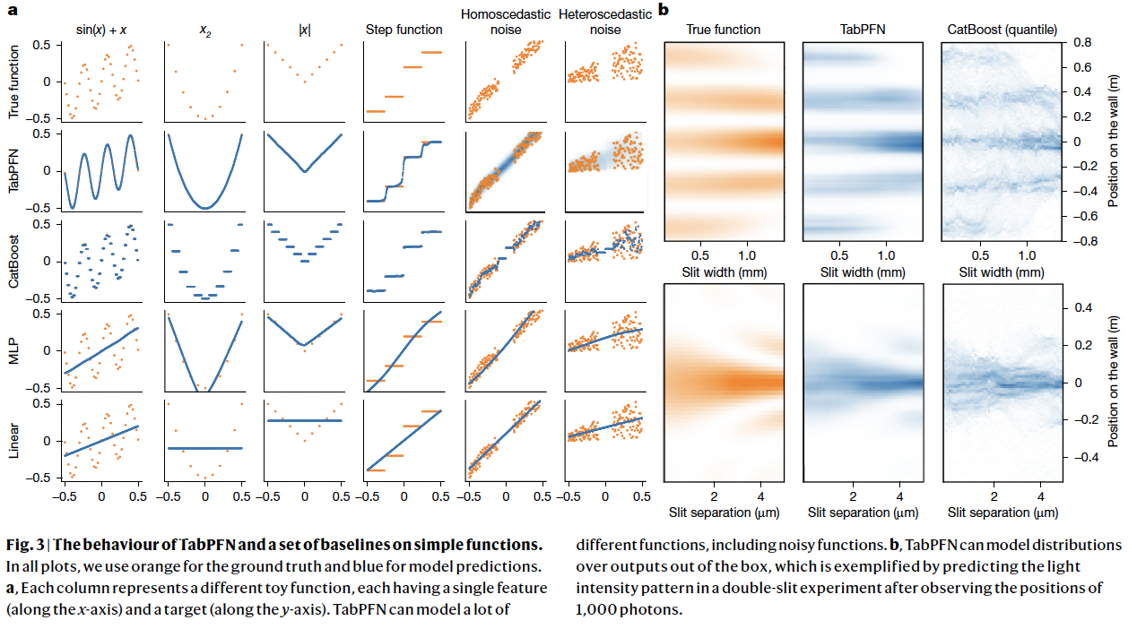
TabPFN vs. (Other) predictors

Results

• Linear (ridge): Can naturally model only linear functions
• MLPs: Perform worse on datasets with highly non-smooth patterns (e.g., Step function)
• CatBoost: Fits only piece-wise constant functions
• TabPFN: Models all!

Main advantage of TabPFN

• Inherent ability to model uncertainty at no extra cost
• Returns a target distribution, capturing the uncertainty of predictions

(2) Figure 3-(b)

Density of light reaching a detector screen in a double-slit experiment (??)

5. Quantitative analysis

Two dataset collections

• AutoML Benchmark
• OpenML-CTR23

Details

• 29 classification datasets
• 28 regression datasets
• Up to 10,000 samples, 500 features and 10 classes

Baseline methods

• Tree-based methods (RF, XGB, CatBoost, LightGBM)
• Linear models
• SVMs
• MLPs

Evaluation metrics

• (Classification) ROC AUC, Accuracy
• (Regression) R\(^2\), Negative RMSE
• Scores were normalized per dataset (1=best \(\leftrightarrow\) 0=worst)

Experimental details

• 10 repetitions with different random seeds
• Train–test splits (90% train, 10% test)
• Hyperparameter tuning
  • Random search with five-fold CV

(1) Comparison with SoTA

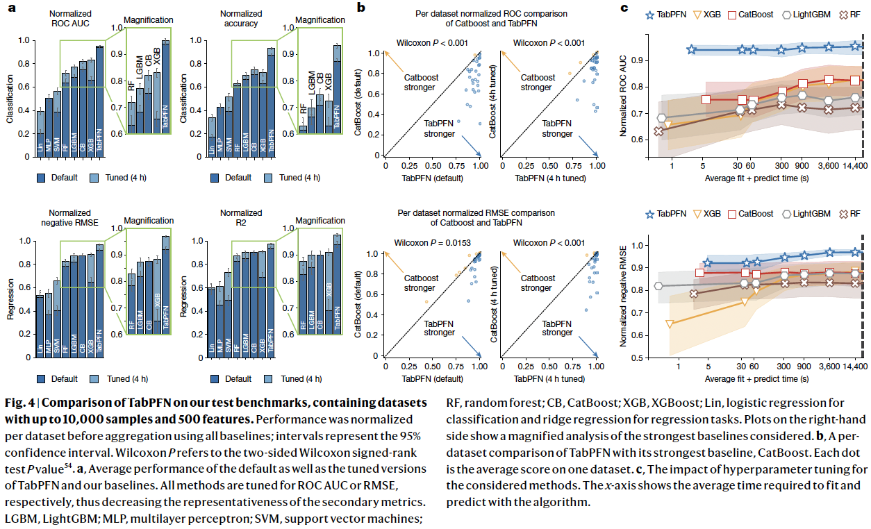
a) Figure 4-(a)

Classifiaction & Regression

b) Figure 4-(b)

Per-dataset comparisons

• Wins on most of the datasets

c) Figure 4-(c)

Shows how the performance of TabPFN and the baselines improve with more time spent on hyperparameter search.

(2) Evaluating diverse data attributes

Robustness of TabPFN to dataset characteristics

( which are traditionally hard to handle for NN-based approaches )

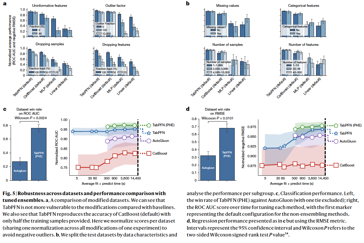
a) Figure 5-(a)

Analysis of the performance across various dataset types

1. Add uninformative features & outliers
   • Very robust to them
2. Drop either samples or features
   • Still outperforms

b) Figure 5-(b)

Split our test datasets into subgroups

Perform analyses per subgroup

Create subgroups based on the …

• (1) Presence of categorical features
• (2) Missing values
• (3) Number of samples
• (4) Number of features

None of these characteristics strongly affect the performance of TabPFN relative to the other methods!

(3) Comparison with tuned ensemble methods

Figure 5-(c),(d)

6. Foundation model with interpretability

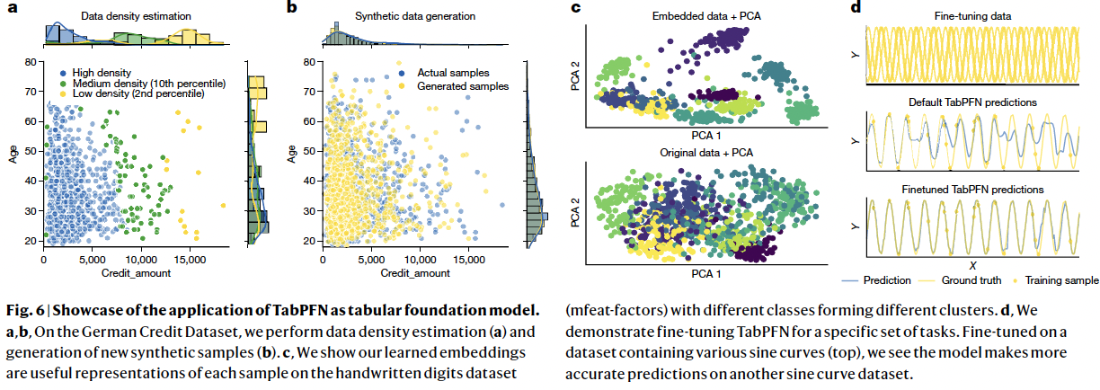
TabPFN exhibits key foundation model abilities!

• e.g., Data generation, density estimation, learning reusable embeddings and fine-tuning

(1) Figure 6-(a)

Estimate the ..

• pdf of numerical features
• pmf of categorical features

Computing the sample densities

\(\rightarrow\) Enables anomaly detection!

(2) Figure 6-(b)

Synthesizing new tabular data samples

\(\rightarrow\) Enables data augmentation or privacy-preserving data sharing

(3) Figure 6-(c)

Yields meaningful feature representations that can be reused for downstream tasks

\(\rightarrow\) Enables data imputation and clustering

(4) Figure 6-(d)

Ability of TabPFN to improve performance through fine-tuning on related datasets

Successfully transfers knowledge even when labels differ significantly between fine-tuning and test tasks

\(\rightarrow\) Enables fine-tuning on specific dataset classes

(5) Interpretation

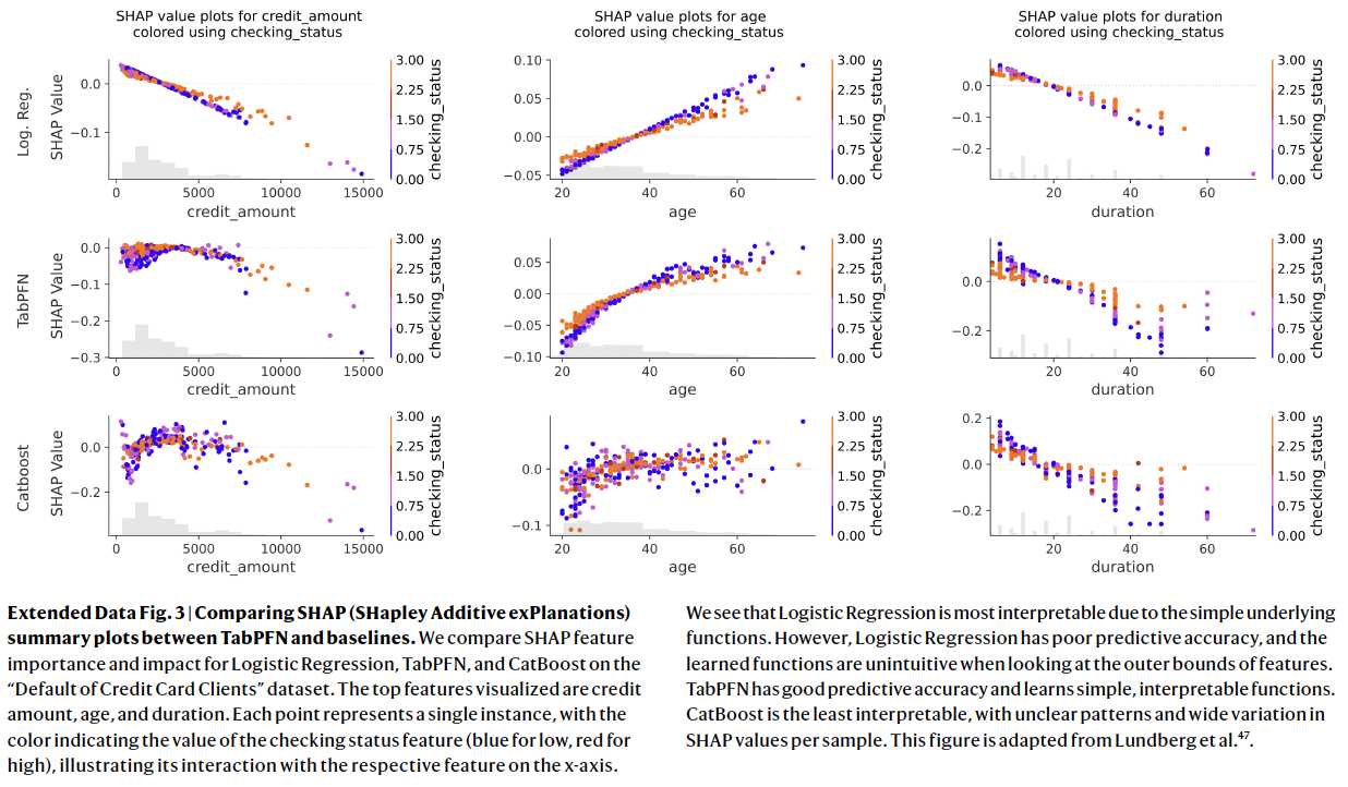
Computation of feature importance through SHAP

• SHAP = Represent the contribution of each feature to the output of the model

Compares the the feature importance and impact for logistic regression, CatBoost and TabPFN

7. Conclusion

TabPFN

• Leverage ICL
• Efficient & Effective
• Up to 10,000 samples and 500 features
• Shift towards foundation models trained on synthetic data o

Potential future directions

• Scaling to larger datasets
• Handling data drift
• …