Relational Graph Transformer

Relational Graph Transformer

Dwivedi, Vijay Prakash, et al. "Relational Graph Transformer." arXiv preprint arXiv:2505.10960 (2025).

arxiv: https://arxiv.org/pdf/2505.10960

Contents

1. Introduction
   1. Relational Deep Learning
   2. Existing gaps
   3. Present work
2. Background
   1. Relational Dl
   2. RDL Methods
   3. Graph Transformers
3. RelGT: Relational Graph Transformers
   1. Tokenization
   2. Transformer Network

Abstract

**Relational Deep Learning (RDL) **

• DL for multi-table relational data
• Treat multi-table relational data as heterogeneous temporal graph

Previous works

• (1) GNN: Suffer in capturing …

  • (1) Complex structural patterns
  • (2) Long-range dependencies

• (2) Graph Transformers

  • Powerful alternatives to GNNs

  • Challenges in applying them to relational entity graphs (REG)?

    • (1) Traditional positional encodings (PE): Fail to generalize to massive, heterogeneous graphs
    • (2) Cannot model the temporal dynamics and schema constraints of relational data
    • (3) Existing tokenization schemes: Lose critical structural information

Proposal: Relational Graph Transformer (RELGT)

• Graph transformer architecture designed specifically for “RELATIONAL” tables
• Two key points
  • (1) “Multi-element tokenization” strategy
  • (2) “Local + Global attention”

(1) “Multi-element tokenization” strategy

• How? Decomposes each node into five components
  • (1) Features + (2) Type + (3) Hop distance + (4) Time + (5) Local structure
• Results: Enables efficient encoding of heterogeneity, temporality, and topology (w/o expensive precomputation)

(2) “Local + Global attention”

• Local attention over sampled subgraphs
• Global attention to learnable centroids

1. Introduction

Real-world enterprise data = Relational DB

• Consist of multiple tables
• Interconnected through primary and foreign keys

Traditional appraoch

• Depended on manual feature engineering within complex ML pipelines

• Require the transformation of multi-table records into flat feature vectors

  \(\rightarrow\) To make it suitable for models (e.g., NN, DT)

(1) Relational Deep Learning

Relational DB = Represented as “relational entity graphs”

• (a) Nodes = Entities
• (b) Edges = Primary-foreign key relationships

\(\rightarrow\) Allows GNNs to learn features directly from the underlying data structure! (w/o feature engineering)

(2) Existing gaps

Limitation of (standard) GNN architectures

• (1) Insufficient structural expressiveness [52, 37, 34]
• (2) Restricted long-range modeling capabilities [1]

Examples)

E-commerce database with three tables

• Customers (green)
• Transactions (blue)
• Products (brown)

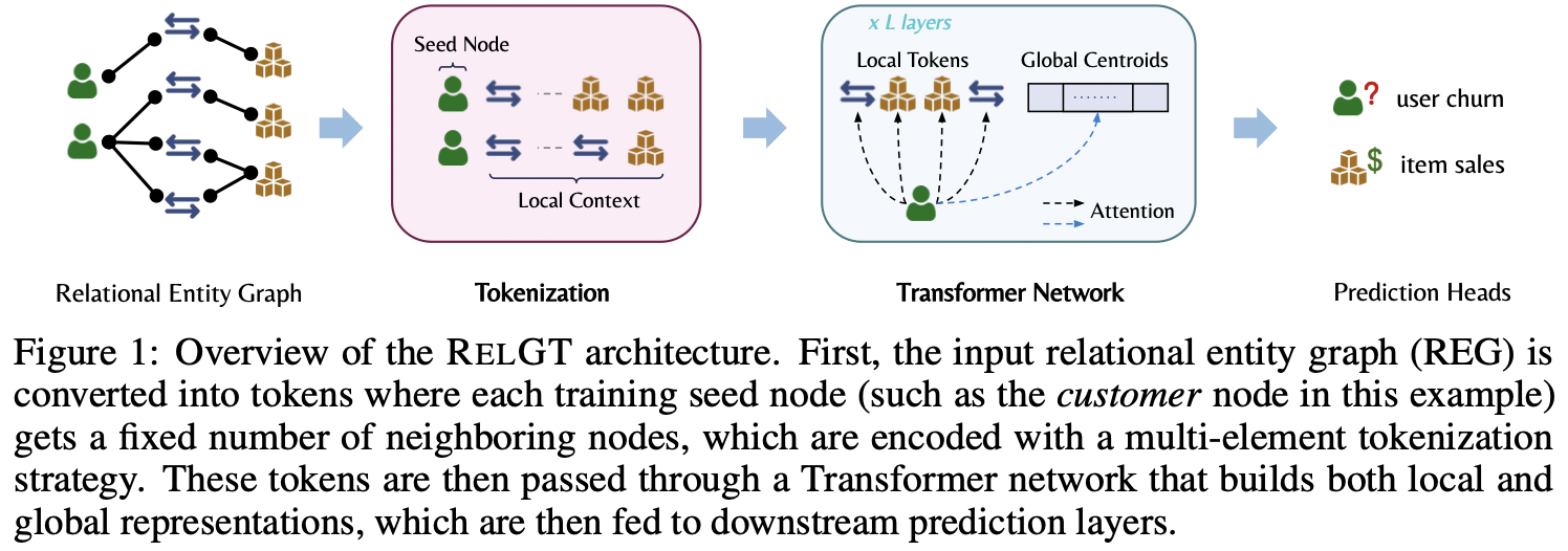
[Figure 1] Relational entity graph

• Standard GNN: Transactions are always two hops away from each other

  (\(\because\) Connected only through shared customers)

• Creates an information bottleneck :(

  • (1) Transaction-to-transaction patterns require multiple layers of message passing
  • (2) Product relationships remain entirely indirect in shallow networks
  • (3) Products would never directly interact in a two-layer GNN

\(\rightarrow\) Inherent structural constraints of GNN architectures that restrict capturing long-range dependencies!!

Solution: **Graph Transformers (GTs) **

• More expressive models for graph learning with (1) & (2)

• (1. Attention) Employ self-attention in the full graph

  \(\rightarrow\) Increase the range of information flow

• (2. PE & SE) Incorporate positional encodings (PE) & **structural encodings (SEs) **

  \(\rightarrow\) Better capture graph topology

Limitation of **Graph Transformers (GTs) **

• Limited to non-temporal / homogeneous / small-scale graphs
• Do not hold for relational entity graphs (REGs)!
• REGs are typically ..
  • (1) Heterogeneous: Different tables representing distinct node types
  • (2) Temporal: Entities often associated with timestamps
  • (3) Large-scale: Containing millions or more records across multiple interconnected tables.

\(\rightarrow\) Render current GTs inadequate for relational DB

(3) Present work (Proposal)

Relational Graph Transformer (RELGT)

First “Graph Transformer” designed for “relational entity graphs”

• a) Goal: Addresses key gaps in existing methods
• b) How: Effective graph representation learning within the RDL framework
• c) Result: Unified model that explicitly captures the temporality, heterogeneity, and structural complexity inherent to relational graphs.

a) Tokenization

Multi-element tokenization scheme

• a) Goal: Converts each node into structurally enriched tokens
  • Five component = node’s features, type, hop distance, time, local structure
• b) How: Sample fixed-size subgraphs as local context windows
• c) Results: Captures fine-grained graph properties (w/o expensive precomputation)

b) Attention

Combines local & global representations

• [Local] Extract features from the local tokens
• [Global] Attend to learnable global tokens that act as soft centroids

c) Validation

Comprehensive evaluation on 21 tasks

2. Background

(1) Relational DL

Converts relational DB \(\rightarrow\) graph structures

• Eliminating the need for feature extraction in multi-table data

a) Definitions

Relational database = Tuple \((T, R)\)

• (1) Collection of tables: \(T = \{T_1, \dots, T_n\}\)
• (2) Inter-table relationships: \(R \subseteq T \times T\)
  • \((T_{\mathrm{fkey}}, T_{\mathrm{pkey}}) \in R\) : Foreign & Primary key (= links)

[Level 1: DB]

• [Level 2: Table] Consists of entities (rows): \(\{v_1, \dots, v_{n_r}\}\)
  • [Level 3: Entity/Row] Consists of
    • (1) Unique identifier (primary key)
    • (2) References to other entities (foreign keys
    • (3) Entity-specific attributes
    • (4) Timestamp information

Structure of relational DB forms a graph representation = Relational entity graph (REG)

REG = Defined as a “heterogeneous” “temporal” graph

• \(G = (V, E, \phi, \psi, \tau)\).
  • \(V\) : Nodes / Entities from the DB tables
  • \(E\) : Edges (representing primary-foreign key relationships)
  • \(\phi\): Maps nodes to their respective types (based on source tables)
  • \(\psi\): Assigns relation types to edges
  • \(\tau\): Captures the temporal dimension (through timestamps)

b) Challenges

REG: exhibit three distinctive properties ( vs. conventional graph data )

1. Schema-defined

• Topology is shaped by primary-foreign key relationships (rather than arbitrary connections)

  \(\rightarrow\) Create specific patterns of information flow

1. Temporal dynamics

• Relational DB track events and interactions over time
  • Need to prevent future information leakage

1. Multi-type heterogeneity

• Different tables = Different entity types with diverse attribute schemas

\(\rightarrow\) These create both challenges & opportunities!!

(2) RDL Methods

Baseline GNN approach for RDL

= Uses a heterogeneous GraphSAGE model with temporal-aware neighbor sampling

Several specialized architectures have been developed to address specific challenges in REG

• RelGNN
  • Introduces composite message-passing with atomic routes to facilitate direct information exchange between neighbors of bridge and hub nodes
• ContextGNN
  • Employs a hybrid approach, combining pair-wise and two-tower representations
• RAG techniques & Hybrid tabular-GNN methods

(3) Graph Transformers

• Extend the self-attention mechanism to graph-structured data
• Powerful alternatives to traditional GNNs
• Typically restrict attention to “local” neighborhoods
• Message-passing networks with attention-based aggregation

3. RelGT: Relational Graph Transformers

(1) Tokenization

Transformers in NLP

Represent text through tokens with Two primary elements

• (1) Token identifiers (features): Denotes the token from a vocabulary set

• (2) Positional encodings (PEs): Represent sequential structure

• E.g., Token = word + positional encoding

Graph Transformers

Also adapt this two-element representation to graphs

• (1) Nodes = Tokens with features
• (2) Graph PEs = Provide structural information

\(\rightarrow\) Works well for homogeneous & static graphs!

Challenges of GTs in REG

• (1) Heterogeneity
• (2) Temporality
• (3) Schema-defined structure

RELGT

Overcomes these limitations!!

a) Sampling and token elements

“Multi-element” token representation approach

• w/o any computational overhead

Single-element vs. Multi-element

• [Single] Compress all structural information into a single PEs

• [Multi] Decompose the token representation into **distinct elements **

  \(\rightarrow\) Allows each component to capture a specific characteristic of REGs

Decomposition

• (1) Node features: Represent entity attributes
• (2) Node types: Encode table-based heterogeneity
• (3) Hop distance: Preserves relative distances among nodes in a local context
• (4) Time encodings: Capture temporal dynamics
• (5) GNN-based PEs: Preserve local graph structure

b) Sampling and token elements

Tokenization: Converts (1) \(G\) \(\rightarrow\) (2) Tokens

• (1) \(G = (V, E, \phi, \psi, \tau)\).
• (2) Sets of tokens (for Transformer input)

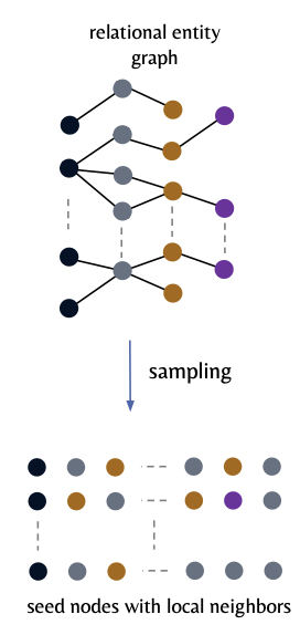
[Figure 2-left]

For each training seed node \(v_i \in V\) ….

Sample a fixed set of \(K\) neighboring nodes \(v_j\)

• Within 2 hops of the local neighborhood

  • Use temporal-aware sampling to prevent temporal leakage

    \(\rightarrow\) Ensure that only nodes with timestamps \(\tau(v_j) \le \tau(v_i)\) are included

• Each token in this set is represented by a 5-tuple

  \((x_{v_j}, \phi(v_j), p(v_i, v_j), \tau(v_j) - \tau(v_i), \mathrm{GNN\text{-}PE}_{v_j})\).

  • (1) Node features \(x_{v_j}\) = Raw features of \(v_j\)
  • (2) Node type \(\phi(v_j)\) = Categorical identifier (= Correspond to the entity’s originating table)
  • (3) Relative hop distance \(p(v_i, v_j)\) = Structural distance btw seed \(v_i\) & neighbor \(v_j\)
  • (4) Relative time \(\tau(v_j) - \tau(v_i)\) = Temporal difference between the neighbor and seed node,
  • (5) Subgraph-based PE \(\mathrm{GNN\text{-}PE}_{v_j}\) = Graph PE for each node within the sampled subgraph
    • Generated by applying a lightweight GNN to the subgraph’s adjacency matrix with random node feature initialization

c) Encoders

Each element in the 5-tuple is processed by a specialized encoder!

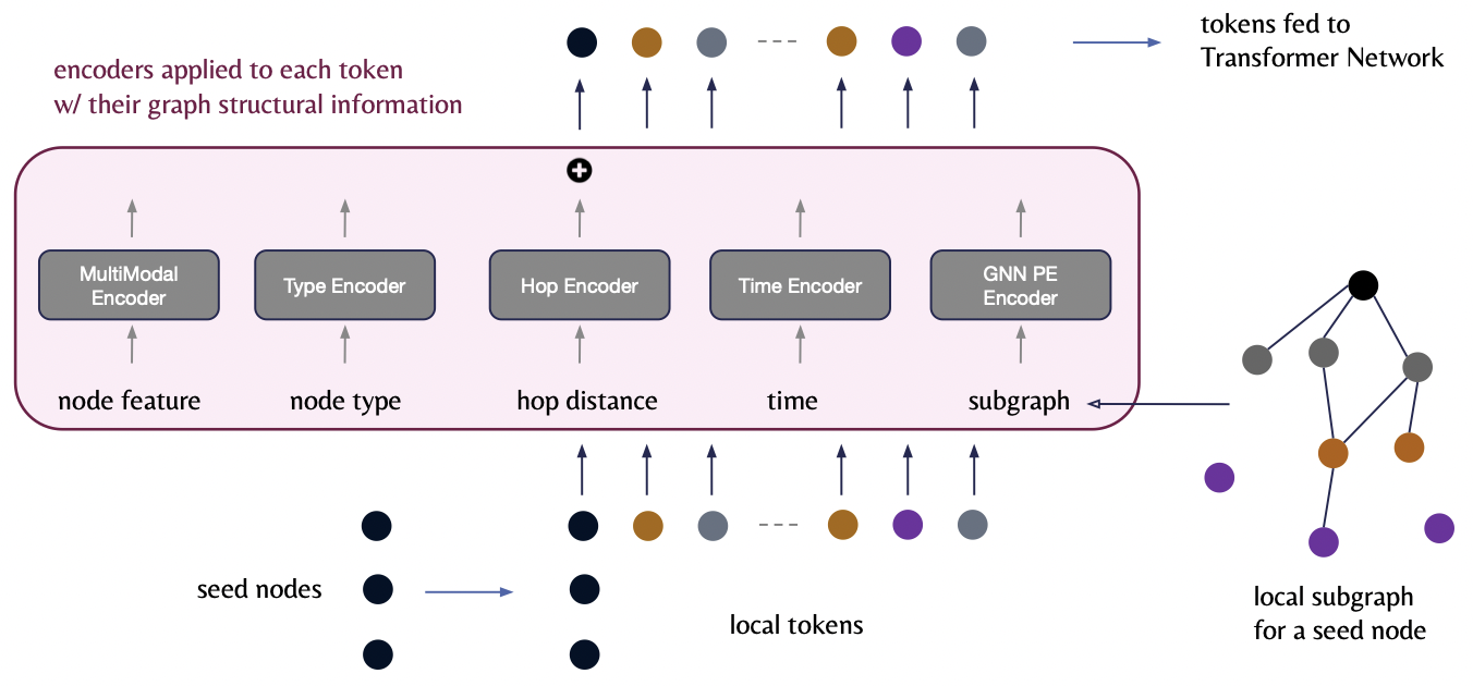
(1) Node Feature Encoder

\[h_{\text{feat}}(v_j) = \text{MultiModalEncoder}(x_{v_j}) \in \mathbb{R}^d\]

• a) Input: Node features \(x_{v_j}\)
  • Table row in DB
  • Representing the columnar attributes of the node \(v_j\) in REG
• b) How: Encode \(x_{v_j}\) into a \(d\)-dim embedding
• Various modalities
  • Each modality (e.g., numerical, categorical, multi-categorical) is encoded separately using modality-specific encoders
• Resulting representations are then aggregated into a unified \(d\)-dim embedding.

(2) Node Type Encoder

\(h_{\text{type}}(v_j) = W_{\text{type}} \cdot \text{onehot}(\phi(v_j)) \in \mathbb{R}^d\).

• a) Input: \(\phi(v_j)\): Node type of \(v_j\)
  • \(W_{\text{type}} \in \mathbb{R}^{d \times \mid T \mid}\): Learnable weight matrix
• b) How: Convert each table-specific entity type \(\phi(v_j)\) to \(d\)-dim representation
• Incorporating the heterogeneous information from the input data

(3) Hop Encoder

\(h_{\text{hop}}(v_i, v_j) = W_{\text{hop}} \cdot \text{onehot}(p(v_i, v_j)) \in \mathbb{R}^d\).

• \(W_{\text{hop}} \in \mathbb{R}^{d \times h_{\max}}\): Learnable matrix mapping hop distances (up to \(h_{\max}\) ).
• \(p(v_i, v_j)\): Relative hop distance that captures the structural proximity
• Encoded into a \(d\)-dim embedding

(4) Time Encoder

\(h_{\text{time}}(v_i, v_j) = W_{\text{time}} \cdot (\tau(v_j) - \tau(v_i)) \in \mathbb{R}^d\).

• \(W_{\text{time}} \in \mathbb{R}^{d \times 1}\): Learnable parameter.
• Linearly transforms the time difference \(\tau(v_j) - \tau(v_i)\)

(5) Subgraph PE Encoder

\(h_{\text{pe}}(v_j) = \text{GNN}(A_{\text{local}}, Z_{\text{random}})_j \in \mathbb{R}^d\).

• \(\text{GNN}(\cdot, \cdot)_j\): Light-weight GNN applied to the local subgraph yielding the encoding for node \(v_j\)
• \(A_{\text{local}} \in \mathbb{R}^{K \times K}\): Adjacency matrix of the sampled subgraph of \(K\) nodes
• \(Z_{\text{random}} \in \mathbb{R}^{K \times d_{\text{init}}}\): Randomly initialized node features for the GNN (with \(d_{\text{init}}\) as the initial feature dimension)
• For capturing local graph structure
• Apply a light-weight GNN to the subgraph
• Effectively preserves important structural relationships…
  • e.g., complex cycles and quasi-cliques between entities
  • e.g., parent-child relationships

d) Final Token Representation

\(h_{\text{token}}(v_j) = O \cdot \left[ h_{\text{feat}}(v_j) \mathbin{\mid \mid } h_{\text{type}}(v_j) \mathbin{\mid \mid } h_{\text{hop}}(v_i, v_j) \mathbin{\mid \mid } h_{\text{time}}(v_i, v_j) \mathbin{\mid \mid } h_{\text{pe}}(v_j) \right]\).

• Combine all encoded elements (with concatenation)
• \(O \in \mathbb{R}^{5d \times d}\): Learnable matrix to mix the embeddings

Summary of multi-element approach

• Comprehensive token representation
• Explicitly captures five components
  • node features, type information, structural position, temporal dynamics, and local topology
  • w/o requiring expensive computation on the graph structure

(2) Transformer Network

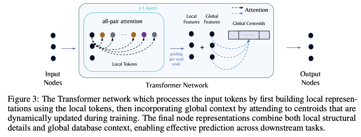
Processes the tokenized REG (from the above) with …

\(\rightarrow\) Combination of LOCAL & GLOBAL attention mechanisms

a) Local module

Goal: Allows each “seed node” to attend to its ”\(K\) local tokens” (which are selected during tokenization)

\(\rightarrow\) Capture the fine-grained relationships defined by the database schema

vs. GNN in RDL in 2 aspects

• (1) Self-attention is used as the message-passing scheme

• (2) Attention is all-pair

  (i.e., All nodes in the local \(K\) set attend to each other)

Details

• \(L\) layer Transformer network

• Provides a broader structural coverage (vs. GNN)

• Example in Section 1) E-commerce
  • Can directly connect seemingly unrelated products
    • by identifying relationships through shared transactions or customer behaviors.
  • Enables the model to capture subtle associations
    • e.g., Customers frequently purchasing unexpected combinations of items

Result: Local node representation \(h_{\text{local}}(v_i)\)

• \(h_{\text{local}}(v_i) = \text{Pool} \left( \text{FFN} \left( \text{Attention}(v_i, \{v_j\}_{j=1}^K) \right) \right)_L\).
  • \(L\): layers
  • FFN and Attention: Standard components in a Transformer
  • Pool: Aggregation of \(\{v_j\}_{j=1}^K\) and \(v_i\) (using a learnable linear combination)

b) Global module

Goal: Enable each seed node to attend to a set of \(B\) global tokens (= representing centroids of all nodes in the graph)

• These centroids are updated during training using an EMA K-Means algorithm applied to seed node features in each mini-batch

\(\rightarrow\) Provide a broader contextual view beyond the local neighborhood.

Result: Global representation \(h_{\text{global}}(v_i)\)

• \(h_{\text{global}}(v_i) = \text{Attention}(v_i, \{c_b\}_{b=1}^B)\).

c) Local + Global

Final output representation (of each node \(v_i\))

= Obtained by combining local and global embeddings

• \(h_{\text{output}}(v_i) = \text{FFN}([h_{\text{local}}(v_i) \mathbin{\mid \mid } h_{\text{global}}(v_i)])\).

d) Downstream prediction

Combined representation (of the seed node)

\(\rightarrow\) Passed through a task-specific prediction head

Trained E2E with task-specific loss functions

https://kumo.ai/research/relational-graph-transformers/