From Similarity to Superiority; Channel Clustering for Time Series Forecasting

From Similarity to Superiority: Channel Clustering for Time Series Forecasting

Contents

1. Abstract
2. Introduction
3. Problem Definition
4. Are Temporal Feature Extractors Effective?
5. Theoretical and Empirical Study on the Linear Mapping
6. Experiments

0. Abstract

CI

• Treat different channels individually
• Leads to poor generalization on unseen instances
• Ignores potentially necessary interactions between channels.

CD

• Mixes all channels with even irrelevant and indiscriminate information
• Results in oversmoothing issues
• Limits forecasting accuracy.

Background

• Lack of channel strategy that effectively balances individual channel treatment for improved forecasting performance without overlooking essential interactions between channels.

Motivation (Observation)

• Correlation between the TS model’s performance boost against channel mixing and the intrinsic similarity on a pair of channels

Proposal: Novel and adaptable Channel Clustering Module (CCM)

• Dynamically groups channels characterized by intrinsic similarities

• Leverages cluster identity ( instead of channel identity )

  $\rightarrow$ Combining the best of CD and CI worlds

1. Introduction

Channel Clustering Module (CCM)

Simultaneously…

• (1) Balances individual channel treatment
• (2) Captures necessary cross-channel dependencies

Motivated by the following key observations

• (1) Both (CI & CD) heavily rely on channel identity information
• (2) Level of reliance is anti-correlated with the similarity between channels (Section 4.1)

$\rightarrow$ CCM thereby involves the strategic clustering of channels into cohesive clusters

• Intra-cluster channels exhibit a higher degree of similarity, effectively replacing channel identity with cluster identity.

• Cluster-aware FFN to ensure individual management of each cluster

• Learns expressive prototype embeddings in the training phase,

  $\rightarrow$ Enable zero-shot forecasting on unseen samples

  ( by grouping them into appropriate clusters )

Summary

• Plug-and-play solution
• 4 different time series backbones (aka. base models)
  • TSMixer (Chen et al., 2023)
  • DLinear (Zeng et al., 2022)
  • PatchTST (Nie et al., 2022)
  • TimesNet (Wu et al., 2022)

2. Related Works

(1) TSF models

pass

(2) Channel Strategies in TSF

CD strategy

• Most DL methods
• Aiming to harness the full spectrum of information across channels.

CI strategy

• Build forecasting models for each channel independently

Comparison (Han et al., 2023; Li et al., 2023a; Montero-Manso & Hyndman, 2021)

• CD = high capacity and low robustness,
• CI = opposite

PRReg (Han et al., 2023)

• Predicting residuals with regularization
• To incorporate a regularization term in the objective to encourage smoothness in future forecasting

$\rightarrow$ However, the essential challenge of channel strategies from the model design perspective has not been solved!

Remains challenging to develop a balanced channel strategy with both high capacity and robustness

[ Prior research ]

Effective clustering of channels to improve the predictive capabilities in diverse applications

• Image classification (Jiang et al., 2010)
• Natural language processing (NLP) (Marin et al., 2023; George & Sumathy, 2023)
• Anomaly detection (Li et al., 2012; Syarif et al., 2012; Gunupudi et al., 2017).
• ex) Traffic prediction (Ji et al., 2023; Liu et al., 2023a)
  • Clustering techniques have been proposed to group related traffic regions to capture intricate spatial patterns.
  • Still, the potential and effect of channel clustering in TSF remain under-explored.

3. Preliminaries

(1) Time Series Forecasting.

• $X=\left[x_1, \ldots \boldsymbol{x}_T\right] \in$ $\mathbb{R}^{T \times C}$
  • $x_t \in \mathbb{R}^C$ .
• $Y=\left[\hat{\boldsymbol{x}}{T+1}, \ldots, \hat{\boldsymbol{x}}{T+H}\right] \in \mathbb{R}^{H \times C}$,
• $X_{[;, i]} \in \mathbb{R}^T$ ( $X_i$ for simplicity ) to denote the $i$-th channel in TS

(2) CI vs. CD

[CI] $f^{(i)}: \mathbb{R}^T \rightarrow \mathbb{R}^H$ for $i=1, \cdots, C$,

[CD] $f: \mathbb{R}^{T \times C} \rightarrow \mathbb{R}^{H \times C}$.

4. Proposed Method

Channel Clustering Module (CCM)

• (1) Model-agnostic method

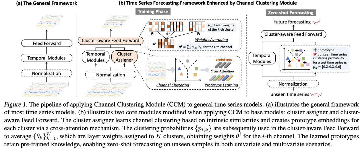
• (2) General TS vs. General TS + CCM: Figure 1

  • 3 components
    • (1) (Optional) Normalization layer
      • (e.g., RevIN (Kim et al., 2021), SAN (Liu et al., 2023c))
    • (2) Temporal modules
      • i.e.) Linear layers, transformer-based, or convolutional backbones,
    • (3) Feed-forward layer
      • forecasts the future values.

(1) Motivation for Channel Similarity

[ Toy experiment ]

Verify the following two assumptions

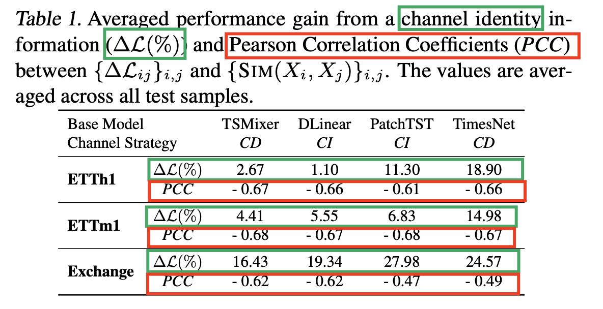
• (1) Existing forecasting methods heavily rely on channel identity information.
• (2) This reliance clearly anti-correlates with channel similarity: for channels with high similarity, channel identity information is less important.

$\rightarrow$ Motivate us to design an approach that provides cluster identity instead of channel identity

• Combining the best of both worlds: high capacity and generalizability

Backbones

• Linear models
  • (1) TSMixer (Chen et al., 2023): CD
  • (2) DLinear: CI
• Transformer-based model
  • (3) PatchTST (Nie et al., 2022): CI
• CNN-based model
  • (4) TimesNet (Wu et al., 2022): CD

Experimental setups

• Train a TS model across all channels

• Evaluate the channel-wise MSE on test set

• Repeat training while randomly shuffling channels in each batch.

  $\rightarrow$ This means channel identity information will be removed

Result: Average performance gain across all channels based on the random shuffling experiments

Summary

• (1) All models rely on channel identity information
• (2) This performance gap anti-correlates with channel similarity

(2) CCM: Channel Clustering Module

a) Channel Clustering

Procedure

• (1) Initialize a set of $K$ cluster embedding $\left{c_1, \cdots, c_K\right}$,

  • where $c_k \in \mathbb{R}^d$

• (2) Each channel $X_i$ is transformed into channel embedding $h_i$ through an MLP

• (3) Probaiblity

  • Prob ( Channel $X_i$ is associated with the $k$-th cluster )

    = Normalized inner-product of the cluster embedding $c_k$ and the channel embedding $h_i$

  • $p_{i, k}=\operatorname{Normalize}\left(\frac{c_k^{\top} h_i}{\left|c_k\right|\left|h_i\right|}\right) \in[0,1]$.

Reparameterization trick (Jang et al., 2016)

• To obtain the clustering membership matrix $\mathbf{M} \in \mathbb{R}^{C \times K}$ ,
  • where $\mathbf{M}{i k} \approx \operatorname{Bernoulli}\left(p{i, k}\right)$.

b) Prototype Learning

Cluster assigner

• Also creates a $d$-dimensional prototype embedding ( for each cluster )

• $\mathbf{C}=\left[c_1, \cdots, c_K\right] \in \mathbb{R}^{K \times d}$: cluster embedding
• $\mathbf{H}=\left[h_1, \cdots, h_C\right] \in \mathbb{R}^{C \times d}$: hidden embedding of the channels

Modified cross-attention

$\widehat{\mathbf{C}}=\text { Normalize }\left(\exp \left(\frac{\left(W_Q \mathbf{C}\right)\left(W_K \mathbf{H}\right)^{\top}}{\sqrt{d}}\right) \odot \mathbf{M}^{\top}\right) W_V \mathbf{H}$.

• where the clustering membership matrix $\mathbf{M}$ is an approximately binary matrix to enable sparse attention on intra-cluster channels specifically

Prototype embedding $\widehat{\mathbf{C}} \in \mathbb{R}^{K \times d}$

• Serves as the updated cluster embedding for subsequent clustering probability

c) Cluster Loss

Further introduce a specifically designed loss function for the clustering quality

Cluster Loss: Incorporates both the

• (1) Alignment of channels with their respective clusters
• (2) Distinctness between different clusters in SSL

Notation

• $\mathbf{S} \in \mathbb{R}^{C \times C}$: Channel similarity matrix
  • with $\mathbf{S}_{i j}=\operatorname{Sim}\left(X_i, X_j\right)$
• ClusterLoss: $\mathcal{L}_C=-\operatorname{Tr}\left(\mathbf{M}^{\top} \mathbf{S M}\right)+\operatorname{Tr}\left(\left(\mathbf{I}-\mathbf{M} \mathbf{M}^{\top}\right) \mathbf{S}\right)$$
  • $\operatorname{Tr}\left(\mathbf{M}^{\top} \mathbf{S M}\right)$ : maximizes the channel similarities within cluster
  • $\operatorname{Tr}\left(\left(\mathbf{I}-\mathbf{M} \mathbf{M}^{\top}\right) \mathbf{S}\right)$: encourages separation between clusters

Final loss function

• $\mathcal{L}=\mathcal{L}_F+\beta \mathcal{L}_C$,

d) Cluster-aware Feed Forward

CI vs CD vs CCM

• CI: Individual Feed Forward per channel

• CD: Shared Feed Forward per channel

• CCM: Cluster-aware Feed Forward

  • Use cluster identity to replace channel identity

Notation

• $h_{\theta_k}(\cdot)$ : the linear layer for the $k$-th cluster
• $Z_i$ : the hidden embedding of the $i$-th channel ( before the last layer )

Final forecast

• Averaged across the outputs of all cluster-aware FFN
  • with $\left{p_{i, k}\right}$ as weights
• $Y_i=\sum_k p_{i, k} h_{\theta_k}\left(Z_i\right)$ for the $i$-th channel.

( For computational efficiency, it is equivalent to $Y_i=h_{\theta^i}\left(Z_i\right)$ with averaged weights $\theta^i=\sum_k p_{i, k} \theta_k$. )