ContiFormer; Continuous-Time Transformer for Irregular Time Series Modeling

ContiFormer: Continuous-Time Transformer for Irregular Time Series Modeling

Contents

1. Abstract
2. Preliminaries
3. Methodology
   1. Overview
   2. Embedding Layer
   3. Mamba Pre-processing Layer
   4. MambaFormer Layer
   5. Forecasting Layer
4. Experiments

0. Abstract

Continuous-time dynamics on Irregular TS (ITS)

• critical to account for (1) data evolution and (2) correlations that occur continuously

Previous works

• a) RNN, Transformer models: discrete

  \(\rightarrow\) Limitations in generalizing to continuous-time data paradigms.

• b) Neural ODEs

  • Promising results in dealing with ITS
  • Fail to capture the intricate correlations within these sequences

ContiFormer

• Extends the relation modeling of Transformer to the continuous-time domain
• Explicitly incorporates the modeling abilities of continuous dynamics of Neural ODEs with the attention mechanism of Transformers.

1. Introduction

Paragraph 1) Characteristics of ITS

• (1) Irregularly generated or non-uniformly sampled observations with variable time intervals
• (2) Still, the underlying data-generating process is assumed to be continuous
• (3) Relationships among the observations can be intricate and continuously evolving.

Paragraph 2) Challenges for moddel design

• Divide into equally sized intervals??

\(\rightarrow\) Weverely damage the continuity of the data

• Recent works)
  • Underlying continuous-time process is appreciated for ITS modeling
• Argue that the correlation within the observed data is also constantly changing over time

Paragraph 3) Two main branches

• (1) Neural ODEs & SSMs
  • Pros) Promising abilities for capturing the dynamic change of the system over time
  • Cons) Overlook the intricate relationship between observations
• (2) RNN & Transformers
  • Pros) Capitalizes on the powerful inductive bias of NN
  • Cons) Fixed-time encoding or learning upon certain kernel functions … fails to capture the complicated input-dependent dynamic systems

Paragraph 4) ContiFormer (Continuous-Time Transformer)

• ContiFormer = (a) + (b)

  • (a) Continuous dynamics of Neural ODEs
  • (b) Attention mechanism of Transformers

  \(\rightarrow\) Breaks the discrete nature of Transformer models.

• Process

  • Step 1) Defining latent trajectories for each observation in the given irregularly sampled data points
  • Step 2) Extends the “discrete” dot-product in Transformers to a “continuous”-time domain
    • Attention: calculated between continuous dynamics.

Contribution

a) Continuous-Time Transformer

• First to incorporate a continuous-time mechanism into attention calculation in Transformer,

b) Parallelism Modeling

• Propose a novel reparameterization method, allowing us to parallelly execute the continuous-time attention in the different time ranges

c) Theoretical Analysis

• Mathematically characterize that various Transformer variants can be viewed as special instances of ContiFormer

d) Experiment Results

• TS interpolation, classification, and prediction

2. Method

Irregular TS

• \(\Gamma=\left[\left(X_1, t_1\right), \ldots,\left(X_N, t_N\right)\right]\),
  • Observations may occur at any time
  • Observation time points \(\boldsymbol{\omega}=\left(t_1, \ldots, t_N\right)\) are with irregular intervals
• \(X=\left[X_1 ; X_2 ; \ldots, X_N\right] \in \mathbb{R}^{N \times d}\).

Input)

• (1) Irregular time series \(X\)
• (2) Sampled time \(\boldsymbol{\omega}\)
  • Sequence of (reference) time points
  • \(t\) : random variable representing a query time point

Output)

• Latent continuous trajectory

  ( = captures the dynamic change of the underlying system )

Summary

• Transforms the discrete observation sequence into the continuous-time domain
• Attention module ( = Continuous perspective )
  • Expands the dot-product operation in vanilla Transformer to the continuous-time domain
    • (1) Models the underlying continuous dynamics
    • (2) Captures the evolving input-dependent process

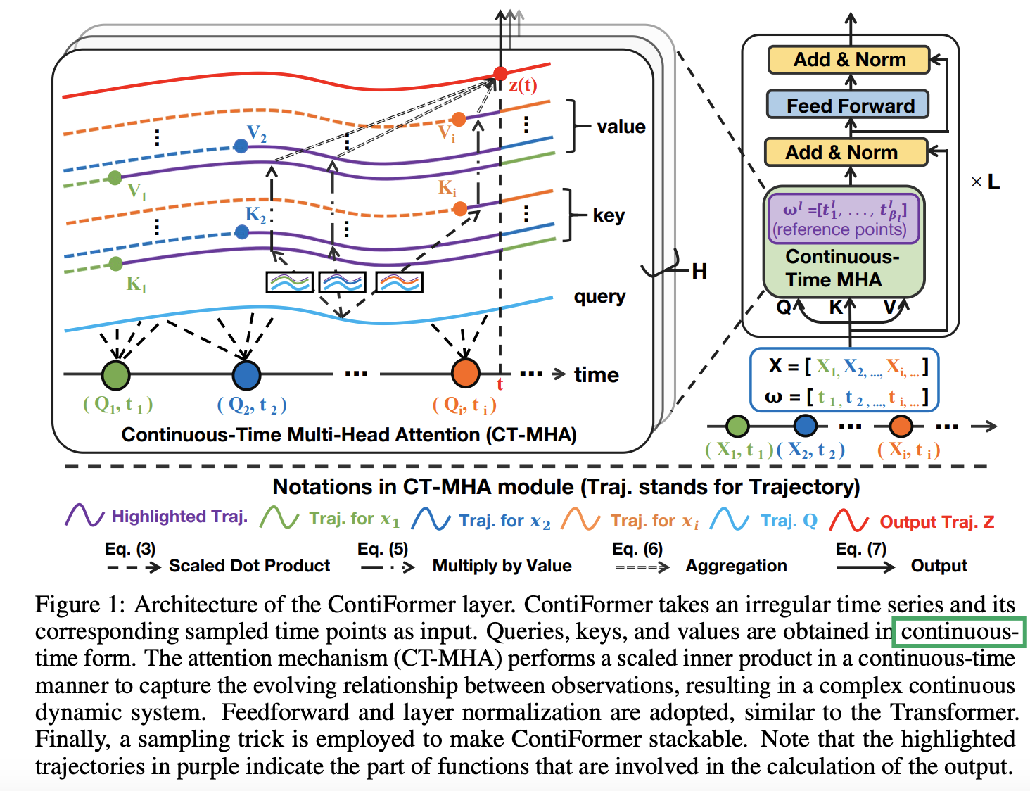
(1) Continuous-Time Attention Mechanism

Core of the ContiFormer layer

• continuous-time multi-head attention (CT-MHA)
• Transform \(X\) into…
  • \(Q=\left[Q_1 ; Q_2 ; \ldots ; Q_N\right]\),
  • \(K=\left[K_1 ; K_2 ; \ldots ; K_N\right]\),
  • \(V=\left[V_1 ; V_2 ; \ldots ; V_N\right]\).
• Utilize ODE to define the latent trajectories for each observation.
  • Latent space: assume that the underlying dynamics evolve following linear ODEs
• Construct a continuous query function
  • by approximating the underlying sample process of the input.

a) Continuous Dynamics from Observations

Attention in continuous form

Step 1) Empoy ODE to define the latent trajectories for each observation

• ex) first observation: at time point \(t_1\)
• ex) last observation: at time point \(t_N\)

Continuous keys and values:

• \(\mathbf{k}_i\left(t_i\right)=K_i\),
  • \(\mathbf{k}_i(t)=\mathbf{k}_i\left(t_i\right)+\int_{t_i}^t f\left(\tau, \mathbf{k}_i(\tau) ; \theta_k\right) \mathrm{d} \tau\).
• \[\mathbf{v}_i\left(t_i\right)=V_i\]
  • \(\mathbf{v}_i(t)=\mathbf{v}_i\left(t_i\right)+\int_{t_i}^t f\left(\tau, \mathbf{v}_i(\tau) ; \theta_v\right) \mathrm{d} \tau\).

Notation:

• \(t \in\left[t_1, t_N\right], \mathbf{k}_i(\cdot), \mathbf{v}_i(\cdot) \in \mathbb{R}^d\):
  • Represent the ODE for the \(i\)-th observation
    • with parameters \(\theta_k\) and \(\theta_v\),
    • with initial state of \(\mathbf{k}_i\left(t_i\right)\) and \(\mathbf{v}_i\left(t_i\right)\)
• \(f(\cdot) \in \mathbb{R}^{d+1} \rightarrow \mathbb{R}^d\):
  • Controls the change of the dynamics

b) Query Function

To model a dynamic system, queries can be modeled as a function of time

• Represents the overall changes in the input

Adopt a common assumption that irregular time series is a “discretization” of an underlying continuous-time process

\(\rightarrow\) Define a closed-form continuous-time interpolation function (e.g., natural cubic spline) with knots at \(t_1, \ldots, t_N\) such that \(\mathbf{q}\left(t_i\right)=Q_i\) as an approximation of the underlying process.

c) Scaled Dot Product

Self-attention

• Calculating the correlation between queries and keys

• By inner product ( \(Q \cdot K^{\top}\) )

Extending the **discrete ** inner-product to its **continuous-time ** domain!!

• Two real functions: \(f(x)\) and \(g(x)\)
• Inner product of two functions in a closed interval \([a, b]\) :
  • \(\langle f, g\rangle=\int_a^b f(x) \cdot g(x) \mathrm{d} x\).
  • Meaning = How much the two functions “align” with each other over the interval

\(\boldsymbol{\alpha}_i(t)=\frac{\int_{t_i}^t \mathbf{q}(\tau) \cdot \mathbf{k}_i(\tau)^{\top} \mathrm{d} \tau}{t-t_i}\).

Evolving relationship between the..

• (1) “\(i\)-th sample” (key)
• (2) “dynamic system” at time point \(t\) (query)
• in a closed interval \(\left[t_i, t\right]\),

\(\rightarrow\) To avoid numeric instability during training, we divide the integrated solution by the time difference

Discontinuity at \(\boldsymbol{\alpha}_i\left(t_i\right)\)…. How to solve?

Define \(\boldsymbol{\alpha}_i\left(t_i\right)\) as …

\(\boldsymbol{\alpha}_i\left(t_i\right)=\lim _{\epsilon \rightarrow 0} \frac{\int_{t_i}^{t_i+\epsilon} \mathbf{q}(\tau) \cdot \mathbf{k}_i(\tau)^{\top} \mathbf{d} \tau}{\epsilon}=\mathbf{q}\left(t_i\right) \cdot \mathbf{k}_i\left(t_i\right)^{\top}\).

d) Expected Values

Query time \(t \in\left[t_1, t_N\right]\),

Value of an observation at time point \(t\): expected value from \(t_i\) to \(t\)

= \(\widehat{\mathbf{v}}_i(t)=\mathbb{E}_{t \sim\left[t_i, t\right]}\left[\mathbf{v}_i(t)\right]=\frac{\int_{t_i}^t \mathbf{v}_i(\tau) \mathrm{d} \tau}{t-t_i}\)

e) Multi-Head Attention

Summary

• Allows for the modeling of complex, time-varying relationships between keys, queries, and values

• Allows for a more fine-grained analysis of data by modeling the input as a continuous function of time

Continuous-time attention ( given a query time \(t\) )

\(\begin{aligned} \operatorname{CT}-\operatorname{ATTN}(Q, K, V, \boldsymbol{\omega})(t) & =\sum_{i=1}^N \widehat{\boldsymbol{\alpha}}_i(t) \cdot \widehat{\mathbf{v}}_i(t) \\ \text { where } \widehat{\boldsymbol{\alpha}}_i(t) & =\frac{\exp \left(\boldsymbol{\alpha}_i(t) / \sqrt{d_k}\right)}{\sum_{j=1}^N \exp \left(\boldsymbol{\alpha}_j(t) / \sqrt{d_k}\right)} \end{aligned}\).

Simultaneous focus on different input aspects

Stabilizes training by reducing attention weight variance

Multi-head: \(\operatorname{CT}-\operatorname{MHA}(Q, K, V, \boldsymbol{\omega})(t)=\operatorname{Concat}\left(\operatorname{head}_{(1)}(t), \ldots, \operatorname{head}_{(\mathrm{H})}(t)\right) W^O\).

(2) Continuous-Time Transformer

\(\begin{aligned} & \tilde{\mathbf{z}}^l(t)=\mathrm{LN}\left(\operatorname{CT}-\operatorname{MHA}\left(X^l, X^l, X^l, \omega^l\right)(t)+\mathbf{x}^l(t)\right) \\ & \mathbf{z}^l(t)=\operatorname{LN}\left(\operatorname{FFN}\left(\tilde{\mathbf{z}}^l(t)\right)+\tilde{\mathbf{z}}^l(t)\right) \end{aligned}\).

a) Sampling Process

ContiFormer layer

• Output: Continuous function \(\mathbf{z}^l(t)\) w.r.t. time as the output
• Input: Discrete sequence \(X^l\)

How to incorporate \(\mathbf{z}^l(t)\) into NN?

\(\rightarrow\) Establish reference time points for the output of each layer

Reference time points

• Used to discretize the layer output
• Correspond to either
  • Input time points (i.e., \(\boldsymbol{\omega}\) )
  • Task-specific time points.

Assume that the reference points for the \(l\)-th layer is \(\boldsymbol{\omega}^l=\left[t_1^l, t_2^l, \ldots, t_{\beta_l}^l\right]\),

\(\rightarrow\) Input to the next layer \(X^{l+1}\) : sampled as \(\left\{\mathbf{z}^l\left(t_j^l\right) \mid j \in\left[1, \beta_l\right]\right\}\)