Frequency Adaptive Normalization For Non-stationary Time Series Forecasting

Abstract
Introduction
FAN
Experiments

0. Abstract

Non-stationarity in TS

(previous) RevIN
- Limited to expressing basic trends
- Incapable of handling seasonal patterns.

\(\rightarrow\) Propose a new instance normalization solution

Frequency adaptive normalization (FAN)

Handles both dynamic trend and seasonal patterns.
Employs the Fourier transform
- To identify instance-wise predominant frequent components
Discrepancy of those frequency components between inputs and outputs

= Explicitly modeled as a prediction task
Model-agnostic method

1. Introduction

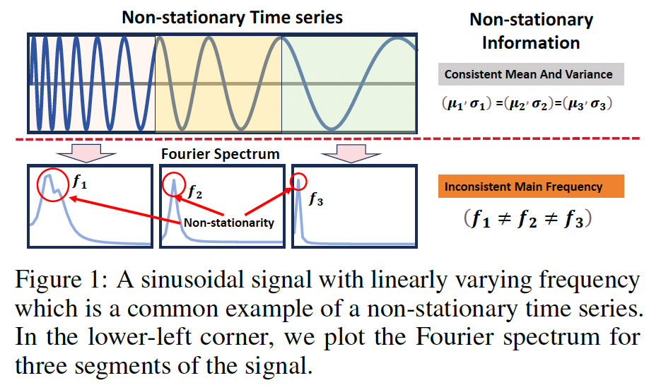
Toy example) Simplest non-stationary signals

Time-variant signal with a gradually damping frequency

Previous methods

Can hardly distinguish this type of change in the time domain.

\(\rightarrow\) Changes in periodic signals can be easily identified with the instance-wise Fourier transform \(\left(f_1 \neq f_2 \neq f_3\right)\).

Principal Fourier components

Provide a more effective representation of non-stationarity

( compared to statistical values )

Frequency Adaptive Normalization (FAN).

Mitigates the impacts from the non-stationarity, by filtering top \(K\) dominant components in the Fourier domain for each input instance,

Can handle unified non-stationary fact

composed of both trend and seasonal patterns.

Removed patterns might evolve from inputs to outputs

\(\rightarrow\) Employ a pattern adaptation module

To forecast future non-stationary information

Contributions

Limitations of RevIN in using temporal distribution statistics

\(\rightarrow\) Introduce FAN, which adeptly addresses both trend and seasonal non-stationary patterns
Explicitly address pattern evolvement with a simple MLP
- Predicts the top \(K\) frequency signals of the horizon series
- Applies these predictions to reconstruct the output.
Apply FAN to four general backbones

2. FAN

Problem Definition

Notation

\(\mathcal{X} \in \mathbb{R}^{N \times D}\),
Task: \(\mathcal{X}_{t-L: t} \rightarrow \mathcal{X}_{t+1: t+H}\),
- where \(\mathcal{X}_{t-L: t} \in \mathbb{R}^{L \times D}\) and \(\mathcal{X}_{t+1: t+H} \in \mathbb{R}^{H \times D}\).
\(\mathbf{X}_t \in \mathbb{R}^{L \times D}\) and \(\mathbf{Y}_t \in \mathbb{R}^{H \times D}\) .

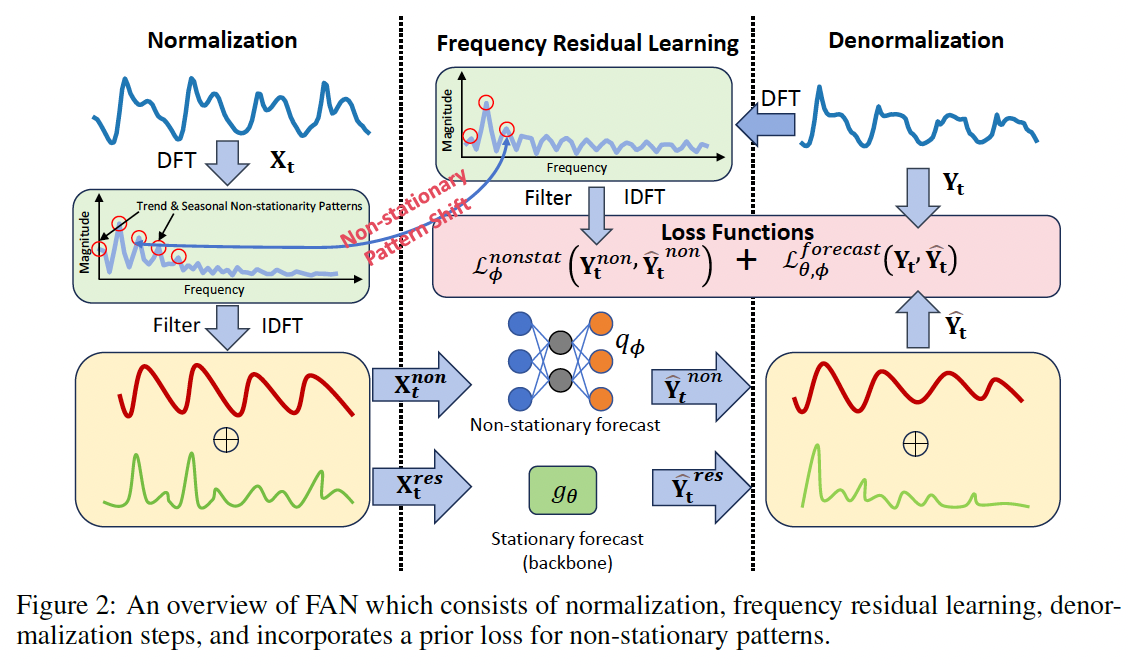
Symmetrically structured instance-wise norm & denorm

(1) Norm: Removes the impacts of non-stationary signals
- Through frequency domain decomposition
(2) Denorm: Addresses potential shifts in frequency components between the input and output
- Supported by a prediction module

(1) Frequency-based Normalization

Removes the top \(K\) dominant components in the frequency domain

Backbone can concentrate on the stationary aspects
Frequency Residual Learning (FRL)
- Apply the FRL to each dimension in a CI manner
- Restores the top \(K\) components into time domain components \(\mathbf{X}_t^{\text {non }}\) with \(\operatorname{IDFT}(\cdot)\).
\(\mathbf{X}_t^{\text {non }}=\operatorname{IDFT}\left(\operatorname{Filter}\left(\mathcal{K}_t, \mathbf{Z}_t\right)\right)\).
- \(\mathbf{Z}_t=\operatorname{DFT}\left(\mathbf{X}_t\right)\), where \(\mathbf{Z}_t \in \mathbb{C}^{T \times D}\)
- \(\mathcal{K}_t=\operatorname{TopK}\left(\operatorname{Amp}\left(\mathbf{Z}_t\right)\right)\).
\(\mathbf{X}_t^{\text{res}}=\mathbf{X}_t-\mathbf{X}_t^{\text{non}}\).

(2) Forecast & Denormalization

\(\hat{\mathbf{Y}}_t=\hat{\mathbf{Y}}_t^{\text {res }}+\hat{\mathbf{Y}}_t^{\text{non}}\).

\(\hat{\mathbf{Y}}_t^{\text {res }}=g_\theta\left(\mathbf{X}_t^{\text {res }}\right)\).
- Forecast backbone model (\(g_\theta\))

\(\hat{\mathbf{Y}}_t^{\text {non }}\): with Non-stationarity shift forecasting

Use a simple MLP model \(q_\phi\) to directly predict future values of the composite top \(K\) frequency components
\[\hat{\mathbf{Y}}_t^{\text {non }}=q_\phi\left(\mathbf{X}_t^{\text {non }}, \mathbf{X}_t\right)=\mathbf{W}_3 \operatorname{ReLU}\left(\mathbf{W}_2 \operatorname{Concat}\left(\operatorname{ReLU}\left(\mathbf{W}_1 \mathbf{X}_t^{n o n}\right), \mathbf{X}_t\right)\right)\]
- Since \(\mathbf{X}_t^{\text {non }}\) only contains top \(K\) frequency information, concatenate the top \(K\) components with the original input \(\mathbf{X}_t\) to handle potential frequency variations.

Loss Functions.

Incorporate a prior guidance loss

For the prediction of principal frequency components

\(\phi, \theta=\underset{\phi, \theta}{\arg \min } \sum_t\left(\mathcal{L}_\phi^{\text {nonstat }}\left(\mathbf{Y}_t^{\text {non }}, \hat{\mathbf{Y}}_t^{\text {non }}\right)+\mathcal{L}_{\theta, \phi}^{\text {forecast }}\left(\mathbf{Y}_t, \hat{\mathbf{Y}}_t\right)\right)\).

\(\mathcal{L}_\phi^{\text {nonstat }}\): Ensures \(q_\phi\) accurately predict the non-stationary principal frequency component
\(\mathcal{L}_{\theta, \phi}^{\text {forecast }}\) : Guarantees that both model optimizes along the overall forecast accuracy