Only the Curve Shape Matters; Training Foundation Models for Zero-ShotMultivariate Time Series Forecasting through Next Curve Shape Prediction

Only the Curve Shape Matters: Training Foundation Models for Zero-Shot Multivariate Time Series Forecasting through Next Curve Shape Prediction

Contents

1. Abstract
2. Introduction
3. Related Works
4. Problem Definition
5. Method
   1. Pretraining Data Preparation
   2. General Time Transformer (GTT)
   3. Why Encoder-only Architecture
6. Experiments

Abstract

General Time Transformer (GTT)

(1) Model

• Encoder-only style foundation model

(2) Downstream Task

• Zero-shot MTS forecasting
• Even surpassing SOTA baselines.

(3) Dataset

• Pretrained on a large dataset of 200M high-quality TS

(4) Pretrain task

• Formulated as a channel-wise next curve shape prediction problem
  • Each TS sample = Sequence of non-overlapping curve shapes with a unified numerical magnitude.

(5) Analysis

• Investigate the impact of ..
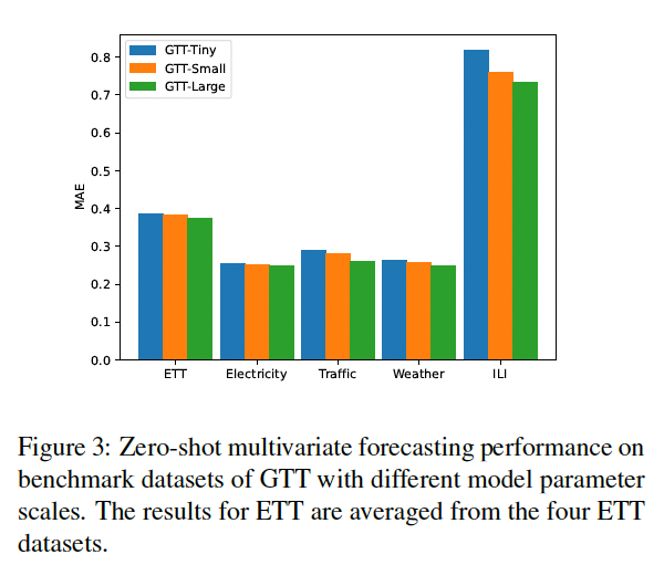
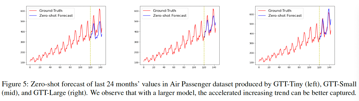
  • (1) varying GTT model parameters
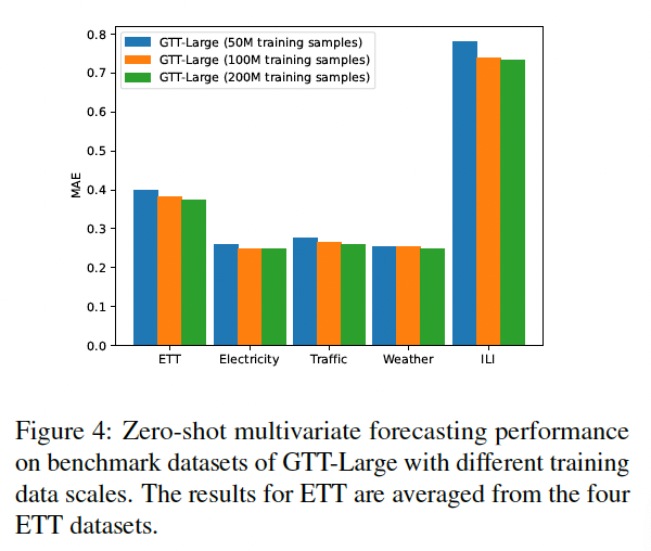
  • (2) training dataset scales
• Observing that the scaling law also holds in the context of zero-shot MTS forecasting

1. Introduction

Transformer-like architecture for TS forecasting

• Pyraformer (Liu et al., 2021), LogTrans (Li et al., 2019), Informer (Zhou et al., 2021), Autoformer (Wu et al., 2021), FEDformer (Zhou et al., 2022), Crossformer (Zhang \& Yan, 2022) and PatchTST (Nie et al., 2022)

Simple MLP-like models

• (Zeng et al., 2023; Ekambaram et al., 2023).

\(\rightarrow\) This discrepancy may be attributed to the fact that Transformers tend to overfit small datasets, and that the largest publicly available time series dataset is less than 10GB (Godahewa et al., 2021)

General Time Transformer (GTT)

• a) Transformer-based foundation model
• b) Zero-shot MTS forecasting on a large dataset containing 200M high-quality time series samples
• c) Formulated as a channel-wise next curve shape prediction problem

Next curve shape prediction problem

• Overcome the challenges of dataset/distribution shift

  & Address varying channel/variable dimensions of TS samples across different domains,

• Each curve shape comprises \(M\) consecutive time points of a single variable.
• Trained to use \(N\) preceding curve shapes as the context

2. Related Works

(1) Transformer

Conjecture: Transformers tend to overfit small datasets

• ex) largest publicly available dataset for TS analysis is less than 10 GB (Godahewa et al., 2021)

To better leverage the powerful modelling ability of Transformers while mitigating the risk of overfitting …

\(\rightarrow\) Reprogramming or fine-tuning pretrained acoustic and LLMs for TS forecasting becomes another promising option (Yang et al., 2021; Zhou et al., 2023; Jin et al., 2023; Chang et al., 2023).

Directly use LLMs for time series forecasting (Gruver et al., 2023).

(2) Foundation models

• ForecastPFN (Dooley et al., 2023)
  • Transformer-based prior-data fitted network
  • Trained purely on synthetic data designed to mimic common time series patterns
• TimeGPT (Garza & Mergenthaler-Canseco, 2023)
  • Transformer-based TS forecasting model
  • Trained over 100B data points, with other data and model details remain unrevealed.

• Lag-Llama (Rasul et al., 2023)

  • Probabilistic TS forecast model adapted from the LlaMA (Touvron et al., 2023)

  • Trained on a large collection of time series from the Monash Time

    Series Repository (Godahewa et al., 2021). PreDcT is a

• PreDcT (Das et al., 2023)
  • patched-decoder style model trained on 1B time points from Google Trends

GTT vs. others

• (1) Training data is much more diverse

  • compared with ForecastPFN, LlaMA and PreDcT.

• (2) Utilize an encoder-only architecture

  • wherein the task of time series forecasting is approached as a problem of predicting the next curve shape in a unified numerical magnitude.

• (3) Incorporates a channel attention mechanism

  • specifically designed for MTS forecasting

    ( rather than focusing solely on univariate forecasting )

3. Problem Definition

We consider building a general purpose zero-shot multivariate time series forecaster that takes in a look-back window of \(L\) time points of a time-series and optionally their corresponding time features as context, and predicts the future \(H\) time points. Let \(\mathbf{x}_{1: L}\) and \(\mathbf{d}_{1: L}\) be the context time series and corresponding time feature values, GTT is a function to predict \(\hat{\mathbf{x}}_{L+1: L+H}\), such that \(\hat{\mathbf{x}}_{L+1: L+H}=f\left(\mathbf{x}_{1: L}, \mathbf{d}_{1: L}\right)\)

Note since we are building a general purpose multivariate forecaster, the only covariates we consider in the pretraining stage are three time features: second of the day, day of the week and month of the year. These three time features, if available, are converted to 6 features using sine and cosine transformations \({ }^2\).

4. Method

(1) Pretraining Data Preparation

a) Size

2.4B univariate or multivariate time points

• From both internal and public sources
• 180,000 univariate or multivariate TS
• Diverse domains
  • including manufacturing, transportation, finance, environmental sensing, healthcare

b) Split

• First 90% time points: training samples
• Remaining 10% time points: validation samples
  • validation loss for early stopping
• Each extracted TS sample consists of 1088 consecutive time points without missing values.

c) Training

• (X) using the preceding 1024 time points
• (Y) predict the values of the last 64 time points

d) Channels

max number of channels for a TS sample to 32

• where 6 channels are reserved for time features

• If # of channels < 32 :
  • set all the values in the added channels to zero
• If # of channels > 32 :
  • divide it into samples with 32 or fewer channels and then supplement the samples with less than 32 channels to reach the total of 32 channels.

e) Normalization

• To achieve a unified numerical magnitude across different datasets
• Normalize each TS sample on a channel-wise basis
• (X,Y)
  • (X) The first 1024 time points are z-score normalized
  • (Y) The last 64 time points are normalized with (X) statistics

\(\begin{aligned} x_{1025: 1088} & =\frac{x_{1025: 1088}-\operatorname{mean}\left(x_{1: 1024}\right)}{\operatorname{stdev}\left(x_{1: 1024}\right)+\epsilon} \\ x_{1: 1024} & =\frac{x_{1: 1024}-\operatorname{mean}\left(x_{1: 1024}\right)}{\operatorname{stdev}\left(x_{1: 1024}\right)+\epsilon} \end{aligned}\).

f) Others

• (filtering) absolute value > 9

• (masking) 1 to 960 time points in the beginning of 10% randomly chosen samples to zero values

  \(\rightarrow\) To generate samples with shorter context lengths,

• (balancing) to ensure balance between the scale and domain diversity of our training data, we restrict the max number of training or validation samples that can be extracted from a single TS to 60,000.

Result

• 200M training samples
• 24M validation samples

(2) General Time Transformer

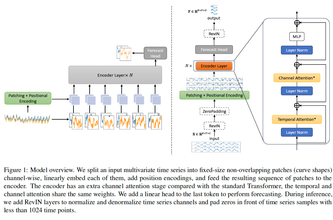
Step 1) Patching

• Split an input MTS into fixedsize non-overlapping patches
  • Each patch = represents a curve shape composed of 64 time points of a single variable
• (inference staeg) RevIN (Kim et al., 2021)

Step 2) Embedding

• Linearly embed each of the patches
• Add position encodings

Step 3) Feed to encoder

• Has an extra channel attention stage
  • For parameter efficiency, the temporal and channel attention share the same weights.

Step 4) Add a linear head to the last token

• to perform forecasting of the next patch (curve shape)

Architectural similarities between GTT & ViT

• curve shapes = special type of image patches
• Difference
  • ViT ) combines RGB channels of an image within its patching process
  • GTT ) independently processes TS channels
    • incorporates an additional stage for channel attention
    • facilitates the learning of cross-variate dependencies with varying channel numbers.

Notation

• \(B\): batch size

• \(T\): input TS length

• \(C\): number of input channels

  (number of target variables, covariates, time features in total)

• \(O\): number of output channels

  (number of target variables)

• \(M\): number of patches
• \(P\): patch size
• \(D\): number of embedding dimensions
• \(N\): number of encoder layers

a) Patching & Positional Encoding

(a-1) Patching

• Input batch: \(\mathbf{X} \in \mathbb{R}^{B \times T \times C}\) \(\rightarrow\) Reshape \(\mathbf{X}\) to \(\hat{\mathbf{X}} \in \mathbb{R}^{B C \times T \times 1}\)
• Conv1D ( k=s=\(P\) , num_filters = \(D\) )
  • to segment input series into patches
  • then embed them into \(M \times D\) dim patch embeddings

(a-2) Positional Encoding

Summary

\[\hat{\mathbf{X}}=\operatorname{Reshape}(\mathbf{X})\]

• \(\mathbf{X} \in \mathbb{R}^{B \times T \times C}\).
• \(\hat{\mathbf{X}} \in \mathbb{R}^{B C \times T \times 1}\).

\(\mathbf{Z}_0=\operatorname{Conv} 1 \mathrm{D}(\hat{\mathbf{X}})+\mathbf{E}_{\text {pos }}\).

• \(\mathbf{E}_{p o s}, \mathbf{Z}_0 \in \mathbb{R}^{B C \times M \times D}\).

b) Encoder Layers

2 MSA

• (1) temporal attention (T-MSA)
• (2) channel attention (C-MSA)

in each encoder layer of GTT

\(\begin{aligned} & \mathbf{Z}_l^{\prime}=\operatorname{T-MSA}\left(\operatorname{LN}\left(\mathbf{Z}_{l-1}\right)\right)+\mathbf{Z}_{l-1}, \quad l=1, \ldots, N \\ & \hat{\mathbf{Z}}_l^{\prime}=\operatorname{Reshape}\left(\mathbf{Z}_l^{\prime}\right), \quad \mathbf{Z}_l^{\prime} \in \mathbb{R}^{B C \times M \times D}, \hat{\mathbf{Z}}_l^{\prime} \in \mathbb{R}^{B M \times C \times D} \\ & \hat{\mathbf{Z}}_l^{\prime \prime}=\operatorname{C-MSA}\left(\operatorname{LN}\left(\hat{\mathbf{Z}}_l^{\prime}\right)\right)+\hat{\mathbf{Z}}_l^{\prime}, \quad l=1, \ldots, N \\ & \mathbf{Z}_l^{\prime \prime}=\operatorname{Reshape}\left(\hat{\mathbf{Z}}_l^{\prime \prime}\right), \quad \hat{\mathbf{Z}}_l^{\prime \prime} \in \mathbb{R}^{B M \times C \times D}, \mathbf{Z}_l^{\prime \prime} \in \mathbb{R}^{B C \times M \times D} \\ & \mathbf{Z}_l=\operatorname{MLP}\left(\operatorname{LN}\left(\mathbf{Z}_l^{\prime \prime}\right)\right)+\mathbf{Z}_l^{\prime \prime}, \quad l=1, \ldots, N \end{aligned}\).

# of channels

• (pretrain) 32

• (inference) vary

  • channel attention requires no positional information!

c) Forecast Head

• Retrieve \(\mathbf{Z}_N^M\) (= last token of the last encoder layer )

• Linear forecast head is attached to \(\mathbf{Z}_N^M\)

  • for predicting the next patch of time points for all channels

    ( i.e., the linear head is shared by all channels )

\(\begin{aligned} & \mathbf{Y}^{\prime}=\mathbf{Z}_N^M W^{D \times P}+\mathbf{b}^P, \quad \mathbf{Z}_N^M \in \mathbb{R}^{B C \times D}, \mathbf{Y}^{\prime} \in \mathbb{R}^{B C \times P} \\ & \mathbf{Y}^{\prime \prime}=\operatorname{Reshape}\left(\mathbf{Y}^{\prime}\right), \quad \mathbf{Y}^{\prime \prime} \in \mathbb{R}^{B \times P \times C} \\ & \mathbf{Y}=\operatorname{Retrieve}\left(\mathbf{Y}^{\prime \prime}\right), \quad \mathbf{Y} \in \mathbb{R}^{B \times P \times O} \end{aligned}\).

d) Loss Function

• Mean Absolute Error (MAE)

  • less sensitive to outliers.

• MAE loss is only calculated on the originally exist data points

  ( i.e., data points in the supplemented channels from the data preparation step are excluded from the loss computation )

e) RevIN and Zero-Padding

RevIN: Only during the inference phase

Zero-Padding: If shorter than 1024, pad zeros at the beginning.

Why? Use of RevIN cannot guarantee a unified magnitude of values for TS!!

ex) with the same curve shapes …

• TS1 [0.0001,0.0002,…,0.1288]
• TS2 [0.001,0.002,…,1.288]

\(\rightarrow\) exact same loss value in our framework!

However, if RevIN were used …

• Contribute different loss values if their original values were used to calculate the loss.

\(\rightarrow\) Discrepancy would introduce bias towards TS samples with larger values during pretraining.

(3) Why Encoder-only Architecture

Encoder-only architecture

• ensures that the predicted values are normalized strictly

However, employing a decoder-only architecture:

• where the first patch predicts the second patch, and subsequently, the first two patches predicts the third patch, the normalization process faces a conflict!!

( Note that normalization is based on the mean and standard deviation of the complete context window )

5. Experiments

(1) Experimental Settings

a) Model Variants

• All models are trained using the 200M training samples and 24M validation samples
• AdamW optimizer
  • training is stopped when the validation loss increases in three consecutive epochs.

b) Benchmark Datasets

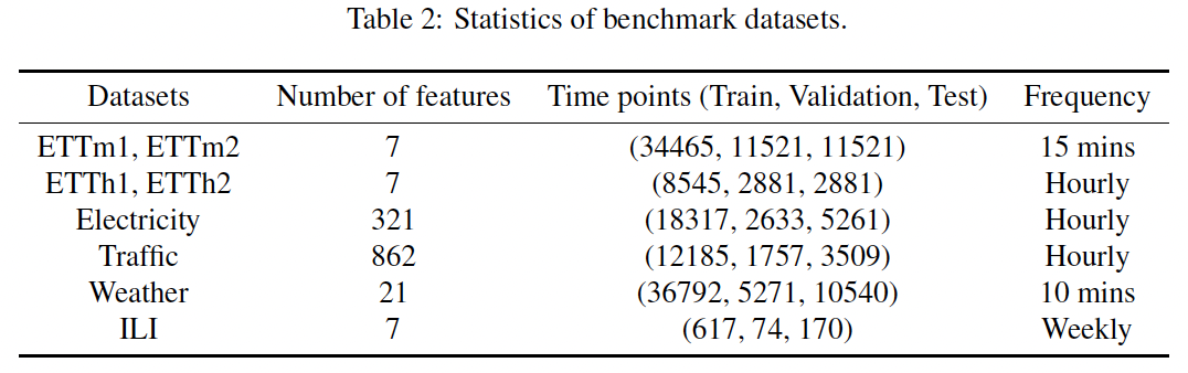
• worthy to mention that all the benchmark datasets are not included in our pretraining data.

(2) Comparison to Supervised Models

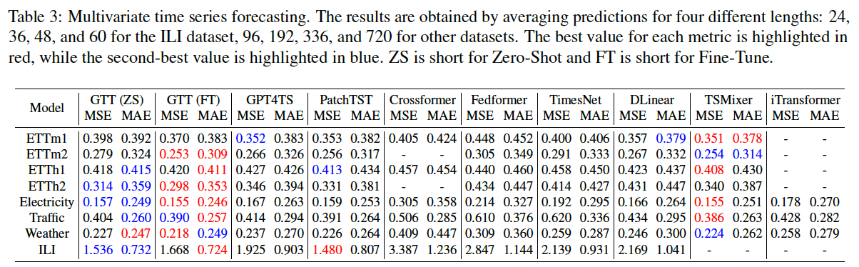
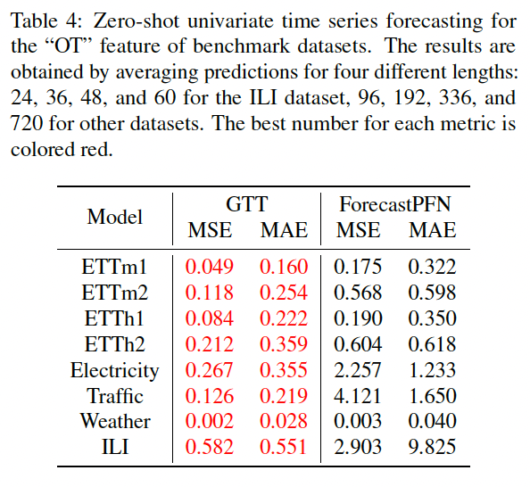
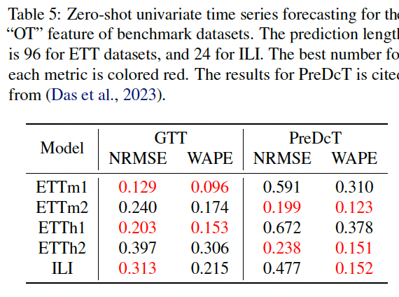
(3) Comparison to Pretrained Models

(4) Scaling Study