GAS-Norm; Score-Driven Adaptive Normalization forNon-Stationary Time Series Forecasting in Deep Learning

GAS-Norm: Score-Driven Adaptive Normalization for Non-Stationary Time Series Forecasting in Deep Learning

Contents

1. Abstract
2. Related Works
3. Proposed Method
   1. Why Adaptive Normalization for a DNN?
   2. Parameter Filtering for Non-stationary Time Series
   3. GAS-Norm
4. Experiments

0. Abstract

Suboptimal performance of DL in TS = By Non-stationarity

This paper:

• (1) Show how DNN fail in simple non-stationary settings
• (2) GAS-Norm
  • For Adaptive TS normalization

Gas-Norm

Based on the combination of

• Generalized Autoregressive Score (GAS)
  • Encompasses a score-driven family of models
  • Estimate the mean and variance at each new observation
  • Provide updated statistics to normalize the input data of the DNN
• DNN
  • Output of the DNN is eventually denormalized
    • Using the statistics forecasted by the GAS model

Leverages the strengths of both statistical modeling and deep

learning.

1. Related Works

(1) Statistical models for non-stationary data

Generalized Autoregressive Score models [8]

• Used for filtering time-varying parameters
  • that update the estimation with the observed score

GAS model is the GARCH model

• Widely used to filter time-varying variance in TS

(2) Recent works

Address challenges caused by non-stationary TS

\(\rightarrow\) Dynamic normalization

Examples

Input normalization [27].

• [23] Batch normalization method for domain adaptation [23]
• [29] DAIN learns the normalization with a nonlinear network
• [10] normalizes the input both in time and frequency

\(\rightarrow\) Ignore non-stationarity over time within the input TS

RevIN [19]

• Denormalization step to restore the statistics removed during the normalization step

[11]

• Adopted a normalization methodology combined with a denormalization step.

• Also consier intra-space shift,

  = Non-stationarity between input & output

• Adopts fixed statistics for the forecast

SAN [24]

• Proposes a dynamic normalization approach

• Splits both input and output into shorter temporal slices, in which non-stationarity can be less impactful

  \(\rightarrow\) Uses them to estimate means and variances

GasNorm (proposed)

• Adapts the statistics online
• Avoids possible problems caused by slices that are…
  • Too long, like non-stationarity
  • Too short, like overly noisy estimations.

2. Proposed Method

(1) Why Adaptive Normalization for a DNN?

DNNs = Composition of many nonlinear functions

\(\rightarrow\) Importance of the stability of the input distribution of each layer has been extensively explored in the literature [18, 21]

GAS-Norm

Improving the generalization of the nonlinear forecasting model in non-stationary settings

Example)

• Complex nonlinear model can be less robust to changes in the input distribution than a linear model when applied to TS data

Toy dataset

TS: Changes in the mean and variance: Can be either

• Predictable (like a simple linear trend)
• Unpredictable (like random regime changes)

Adaptive and flexible way to filter the location and scale parameters of our data online

\(\rightarrow\) Allow us to normalize the data even in the presence of deterministic or unpredictable non-stationarity

(2) Parameter Filtering for Non-stationary Time Series

Forecasting problem

• \(E\left[Y_{t+h} \mid X_t, \ldots, X_{t-l} ; w\right]=f_w\left(X_t, \ldots, X_{t-l}\right)\).
• Conditional expectation
  • Random variable that depends on the realizations of \(\left\{X_t, \ldots, X_{t-l}\right\}\).

Input distribution at time \(t\) of a \(k\)-dim input vector

• Unknown joint distribution of all input features
• \(P_{X_t}\left(x_t\right)=P_{X_{1, t}, X_{2, t}, \ldots X_{k, t}}\left(x_{1, t}, x_{2, t}, \ldots x_{k, t}\right)\),

Stationary case

• (mean, var) of the input distn = constant

Non-stationary case

• (mean, var) of the input distn = change in time

Assume to know the type of parametrized density function of the marginal distributions of each input feature, conditional to the past observations of that feature itself.

• ex) Gaussian distribution with time-varying mean and variance
  • \(P_{X_{i, t} \mid \mathcal{F}_{i, t}}\left(x_{i, t}\right)=\mathcal{N}\left(\mu_{i, t}, \sigma_{i, t}^2\right)\).

Observation-driven state-space representation

Realizations of our input feature \(x_{i, t}\) are given by:

\(\begin{aligned} & x_{i, t}=\mu_{i, t}+\sigma_{i, t} \epsilon_{i, t} \\ & \mu_{i, t}=g\left(\mu_{i, t-1}, x_{i, t-1}\right) \\ & \sigma_{i, t}^2=g^{\prime}\left(\sigma_{i, t-1}^2, x_{i, t-1}\right) \end{aligned}\).

Notation

• \(\theta_t=\left[\mu_t, \sigma_t^2\right]\) = Time-varying parameter vector

  ( Drop the feature index \(i\). )

Modify the GAS formulation in [22]

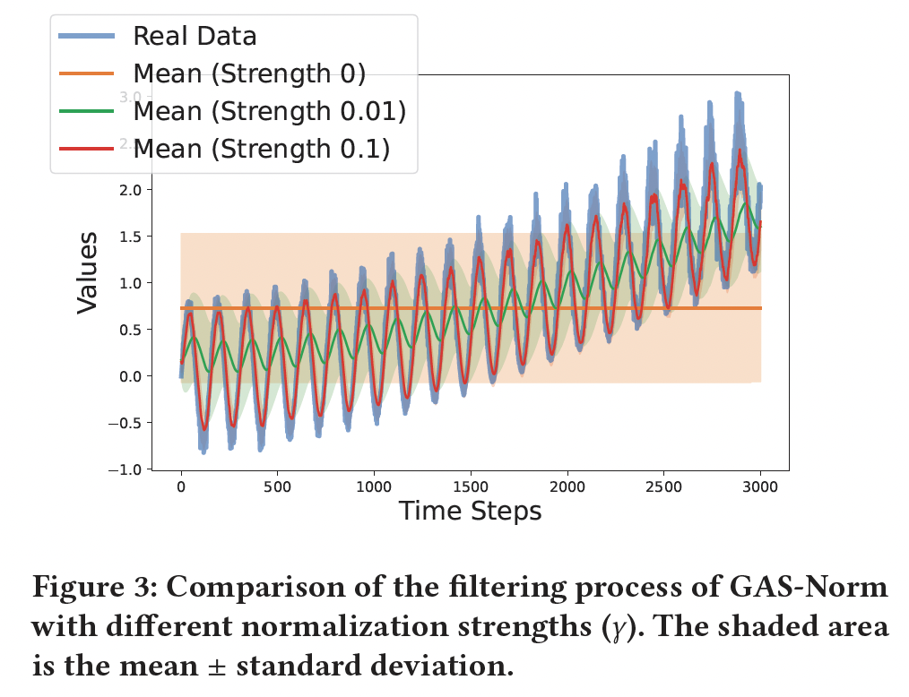
By adding a new hyperparameter \(\gamma \in[0,1)\)

• Control how much importance is given to
  • (1) maximizing the likelihood
  • (2) keeping the parameter stable
• Controls the update speed of the normalization parameters
• Low values = Slow adaptation
  • Normalized input more similar to the original one
  • (Extreme) \(\gamma=0\) : Equivalent to a static normalization.
• \(\max _\theta \gamma \log p\left(x_t \mid \theta\right)-\frac{1-\gamma}{2} \mid \mid \theta-\theta_{t \mid t-1} \mid \mid _{P_t}^2\).
  • where \(P_t\) is a penalization matrix

First-order Taylor expansion:

• \(\log p\left(x_t \mid \theta\right)=\log p\left(x_t \mid \theta_{t \mid t-1}\right)+\left(\theta-\theta_{t \mid t-1}\right) \nabla_\theta\left(x_t \mid \theta_{t \mid t-1}\right)\).
• First-order condition
  • \(\theta_{t \mid t}=\theta_{t \mid t-1}+\frac{\gamma}{1-\gamma} P_t^{-1} \nabla_\theta\left(x_t \mid \theta_{t \mid t-1}\right)\).

Summary

• (Update) \(\theta_{t \mid t}=\theta_{t \mid t-1}+\frac{\gamma}{1-\gamma} \alpha \tilde{\nabla}_\theta\left(x_t \mid \theta_{t \mid t-1}\right)\).
• (Linear prediction) \(\theta_{t+1 \mid t}=\omega+\beta \theta_{t \mid t}\)
• Parameters = \((\alpha, \beta, \omega)\)

To optimize these static parameters…

• Prediction error decomposition

  \(p\left(x_1, x_2, \ldots, x_T\right)=p\left(x_T \mid x_{T-1}\right) \ldots p\left(x_2 \mid x_1\right) p\left(x_1\right)\).

New optimization problem

\(\begin{aligned} \max _{\alpha, \omega, \beta} & \gamma \log p\left(x_1\right)-\frac{1-\gamma}{2} \mid \mid \theta_1-\theta_0 \mid \mid _{P_t}^2+ \\ & \sum_{t=2}^T \gamma \log p\left(x_t \mid x_{t-1}\right)-\frac{1-\gamma}{2} \mid \mid \theta_t-\theta_{t \mid t-1} \mid \mid _{P_t}^2 \end{aligned}\),

Find optimal \(\alpha, \beta, \gamma\)

• Use them to filter the mean and variance
• Normalize the marginal distribution of each feature at each time step

Joint input distribution:

\(\begin{aligned} & P_{\tilde{X}_{1, t}, \tilde{X}_{2, t}, \ldots \tilde{X}_{k, t}}\left(\tilde{x}_{1, t}, \tilde{x}_{2, t}, \ldots \tilde{x}_{k, t}\right)= \\ & p\left([0,0, \ldots 0],\left[\begin{array}{ccc} 1 & \operatorname{Corr}\left(x_{1, t}, x_{2, t}\right) & \ldots \\ \operatorname{Corr}\left(x_{1, t}, x_{2, t}\right) & 1 & \ldots \\ \ldots & \ldots & 1 \end{array}\right]\right) \end{aligned}\).

• mean zero and a covariance matrix equal to the correlation matrix of the original joint distribution
• Normalized features can be used as input for a DNN

(3) GAS-Norm

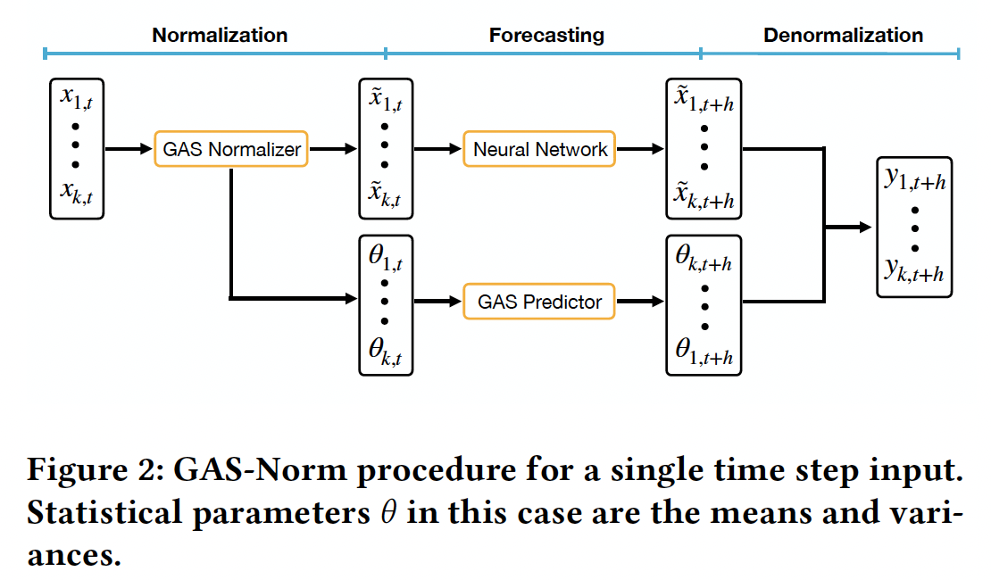
Different blocks

• (1) Normalization
• (2) Forecasting
• (3) Denormalization

\(y_{i, t+h} =\mu_{i, t+h}+\sigma_{i, t+h} e_{i, t+h}\).

• \(\mu_{i, t+h} =g\left(\mu_{i, t+h-1}\right)\).
• \(\sigma_{i, t+h}^2 =g^{\prime}\left(\sigma_{i, t+h-1}^2\right)\).
• \(e_{i, t+h} =f_w\left(\tilde{X}_t, \ldots, \tilde{X}_{t-l}\right)+\epsilon_{i, t+h}\).
  • DNN = Residual Learning

a) Normalization

\(\begin{aligned} & \mu_{t+1}=\omega_\mu+\beta_\mu\left[\frac{\gamma}{1-\gamma} \alpha_\mu \frac{y_t-\mu_t}{1+\frac{\left(y_t-\mu_t\right)^2}{v \sigma_t^2}}+\mu_t\right] \\ & \sigma_{t+1}^2=\omega_\sigma+\beta_\mu\left[\frac{\gamma}{1-\gamma} \alpha_\sigma\left(\frac{(v+1)\left(y_t-\mu_t\right)^2}{v+\frac{\left(y_t-\mu_t\right)^2}{\sigma_t^2}}-\sigma_t^2\right)+\sigma_t^2\right] \end{aligned}\).

b) Forecasting & Denormalization

\(\begin{aligned} \mu_{t+1} & =\omega_\mu+\beta_\mu \mu_t \\ \sigma_{t+1}^2 & =\omega_\sigma+\beta_\sigma \sigma_t^2 \end{aligned}\).

Summary

Autoregressive approach

• Prediction is assumed as real observation to predict the next step.

• Forecast by DNN is combined with the means and variances predicted by the GAS

  \(\rightarrow\) Re-introducing the information removed during the normalization procedure

3. Experiments