KAN4TSF; Are KAN and KAN-based models Effective for Time Series Forecasting?

KAN4TSF: Are KAN and KAN-based models Effective for Time Series Forecasting?

Contents

1. Abstract
2. Introduction

3. Problem Definition

4. KAN

5. RMoK

0. Abstract

Existing methods in TS: 2 challenges

• (1) Mathematical theory of mainstream DL-based methods does not establish a clear relation between network sizes and fitting capabilities
• (2) Lack interpretability

KAN in TS forecasting

Better (1) mathematical properties and (2) interpretability

Propose Reversible Mixture of KAN experts (RMoK)

= Uses a mixture-of-experts structure to assign variables to KAN experts.

https://github.com/2448845600/KAN4TSF.

1. Introduction

Universal approximation theorem (UAT)

• Cannot provide a guarantee on the necessary network sizes (depths and widths) to approximate a predetermined continuous function with specific accuracy

Kolmogorov-Arnold Network (KAN)

• Based on the Kolmogorov-Arnold representation theorem (KART)

  • (1) Proves that a multivariate continuous function can be represented as a combination of finite univariate continuous functions

    • Establishes the relationship between

      • a) network size

      • b) input shape

        under the premise of representation

  • (2) Offers a pruning strategy

    • Simplifies the trained KAN into a set of symbolic functions

    • Enables the analysis of specific modules’ mechanisms

      \(\rightarrow\) Enhance the network’s interpretability

KAN’s function fitting idea

= Consistent with the properties of TS (i.e., periodicity, trend)

(1) KAN

= Employs a trainable 1D B-spline functions

• to convert incoming signals

(2) KAN’s variants:

= Replace the B-splines with

• Chebyshev polynomials
• wavelet functions
• Jacobi polynomials
• ReLU functions

to accelerate training speed and improve performance.

(3) Other studies:

= Introduce KAN with existing popular network structures for various applications.

• ConvKAN
• GraphKAN

Existing studies lack a KAN-based model that considers TS domain knowledge!!

Proposal: RMoK

KAN-based model for the TS forecasting

Evaluate its effectiveness from 4 perspectives

• (1) Performance
• (2) Integration
• (3) Speed
• (4) Interpretability.

Reversible Mixture of KAN Experts model (RMoK)

• Multiple KAN variants

  • Use as experts

• Gating network

  • Adaptively assign variables to specific experts

• Implemented as a single-layer network

  ( \(\because\) Hope that it can have similar performance and better interpretability than existing methods )

2. Problem Definition

• Input: \(\mathcal{X}=\left[X_1, \cdots, X_T\right] \in \mathbb{R}^{T \times C}\),

• Ouptut: \(\mathcal{Y}=\left[X_{T+1}, \cdots, X_{T+P}\right] \in \mathbb{R}^{P \times C}\)

3. KAN

Kolmogorov-Arnold representation theorem (KART)

• Mathematical foundation of the KAN

• Makes KAN more fitting and interpretable than MLP

  ( MLP: based on the universal approximation theorem )

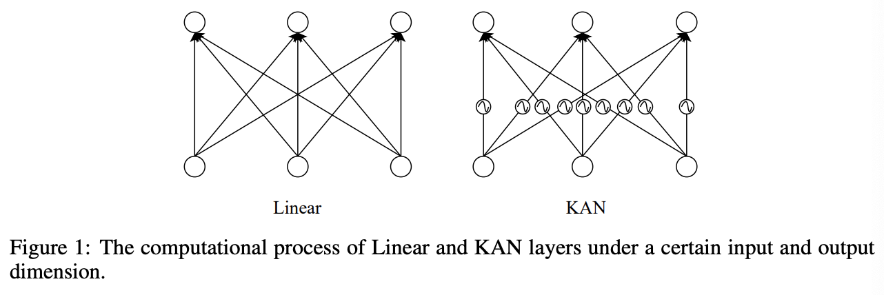
Dfference between KAN and MLP

\(\mathrm{KAN}(\mathbf{x})=\left(\mathbf{\Phi}_L \circ \mathbf{\Phi}_{L-1} \circ \cdots \circ \mathbf{\Phi}_2 \circ \mathbf{\Phi}_1\right) \mathbf{x}\).

• Input tensor \(\mathbf{x} \in \mathbb{R}^{n_0}\) & Structure of \(L\) layers

• \(\boldsymbol{\Phi}_l, l \in[1,2, \cdots, L]\): KAN layer
• Output dimension of each KAN layer: \(\left[n_1, n_2, \cdots, n_L\right]\).

Transform process of \(j\)-th feature in \(l\)-th layer

• \[\mathbf{x}_{l, j}=\sum_{i=1}^{n_{l-1}} \phi_{l-1, j, i}\left(\mathbf{x}_{l-1, i}\right), \quad j=1, \cdots, n_l\]

• \(\phi\) consists two parts:

  \(\phi(x)=w_b \operatorname{SiLU}(x)+w_s \operatorname{Spline}(x)\).

  • (1) Spline function
    • \(\operatorname{Spline}(\cdot)\): linear combination of B-spline functions
    • \(\operatorname{Spline}(x)=\sum_i c_i B_i(x)\).
  • (2) Residual activation function
    • with learnable parameters \(w_b, w_s\)

4. RMoK

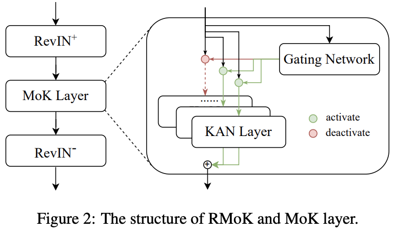
(1) Mixture of KAN Experts Layer

Mixture of KAN experts (MoK) layer

• KAN + Mixture of experts (MoE)
• Uses a gating network to assign KAN layers to variables according to temporal features

KAN & KAN variants

• Only differ in the spline function

  \(\phi(x)=w_b \operatorname{SiLU}(x)+w_s \operatorname{Spline}(x)\).

This paper

• Use \(\mathcal{K}(\cdot)\) to represent these methods uniformly

• MoK layer with \(N\) experts:

  \(\mathbf{x}_{l+1}=\sum_{i=1}^N \mathcal{G}\left(\mathbf{x}_l\right)_i \mathcal{K}_i\left(\mathbf{x}_l\right)\).

  • where \(\mathcal{G}(\cdot)\) is a gating network

• Adapt to the diversity of TS

  • Each expert learning different parts of temporal features

Gating network

• Key module of the MoK layer

• Responsible for learning the weight of each expert from the input data.

• Softmax gating network \(\mathcal{G}_{\text {softmax }}\)

  • Uses a softmax function & learnable weight matrix \(\mathbf{w}_g\)
  • \(\mathcal{G}_{\text {softmax }}(\mathbf{x})=\operatorname{Softmax}\left(\mathbf{x w}_g\right)\).

• However, it activates all experts once

  \(\rightarrow\) Resulting in low efficiency ( when there are a large number of experts )

  \(\rightarrow\) Adopt the sparse gating network

Sparse gating network

\(\begin{gathered} \mathcal{G}_{\text {sparse }}(\mathbf{x})=\operatorname{Softmax}(\operatorname{KeepTopK}(H(\mathbf{x}), k)) \\ H(\mathbf{x})=\mathbf{x w}_g+\operatorname{Norm}\left(\operatorname{Softplus}\left(\mathbf{x w}_{\text {noise }}\right)\right) \end{gathered}\).

• Only activates the best matching top- \(k\) experts.
• Adds Gaussian noise to input time series by \(\mathbf{w}_{\text {noise }}\) & KeepTopK operation to retains experts with the highest \(k\) values.

(2) Reversible Mixture of KAN Experts Model

Sophisticated KAN-based model

=> By stacking multiple KANs

( or replacing the linear layers of the existing models with KANs. )

Design a simple KAN-based model

• Easy to analyze
• Achieve comparable performance to the most SOTA TS models

Propose a simple, effective and interpretable KAN-based model,

Reversible Mixture of KAN Experts Network (RMoK)

[Training stage]

• Gating network has a tendency to reach a winner-take-all state

  = Gives large weights for the same few experts

• ( Following the previous work ) Load balancing loss function

  • Encourage experts have equal importance

Load balancing loss function

• Step 1) Count the weight of experts as loads,
• Step 2) Calcuate the square of the coefficient of variation
  • \(\mathrm{L}_{\text {load-balancing }}=\mathrm{CV}(\text { loads })^2\).

Total loss function

• \(\mathrm{L}=\operatorname{MSE}(\mathcal{Y}, \hat{\mathcal{Y}})+w_l \cdot \mathrm{~L}_{\text {load-balancing }}\).