MCformer; MTS Forecasting with Mixed-Channels Transformer

MCformer: Multivariate Time Series Forecasting with Mixed-Channels Transformer

Contents

1. Abstract
2. Introduction
3. Method

0. Abstract

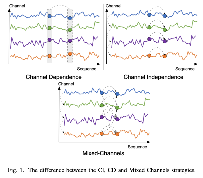
Channel Dependence (CD)

• Treats each channel as a univariate sequence

Channel Independence (CI)

• Treats all channels as a single channel
• Challenge of interchannel correlation forgetting

MCformer

(MTS forecasting model with mixed channel features)

• Innovative Mixed Channels strategy
• Combine the
  • (1) Data expansion advantages (of the CI strategy)
  • (2) Ability to counteract inter-channel correlation forgetting
• Details:
  • Blends a specific number of channels
  • Attention mechanism to effectively capture inter-channel correlation information

1. Introduction

Success of the CI strategy

• DLinear: has surpassed existing models !
• PatchTST: CI strategy model
  • Expanding the dataset and enhancing the model’s generalization capability

Research on PETformer

• CI > CD, because multivariate features can interfere with the extraction of long sequence features.
• This result goes against intuition, as in DL, more information typically improves model generalization.

Two main reasons why CI >CD

1. Can expand the dataset to improve the generalization performance of the model ( feat. PatchTST )
2. Can avoid the destruction of long-term feature information by channel-wise correlation information ( feat. PETformer )

Drawbacks of CI strategy

• Overlook inter-channel feature information
• With large # of channels, there may be an issue of inter-channel correlation forgetting

Mixed Channels strategy

• (CI) Retains the advantages of the CI strategy in expanding the dataset
• (CD) Avoiding the disruption of longterm feature information by channels.
• Addresses the issue of inter-channel correlation forgetting.

MCformer

• Multi-channel TS forecasting model with mixed channel features.
• Procedure
  • Step 1) Expands the data using the CI strategy
  • Step 2) Mixes a specific number of channels
  • Step 3) Attention mechanism
    • Capture the correlation information between channels
  • Step 4) Encoder result is unflattened to obtain the predicted values of all channels

2. Method

(1) Problem Definition

Input: \(X=\left\{\mathbf{x}_1, \mathbf{x}_2, \ldots, \mathbf{x}_t\right\} \in \mathbb{R}^{t \times M}\),

• \(\mathbf{x}_t=\left[x_t^1, x_t^2, \ldots, x_t^M\right]^{\top}\).

Target: \(\left\{\mathbf{x}_{t+1}, \ldots, \mathbf{x}_{t+h}\right\}\)

Incorporate a Mixed-Channels Block into the vanilla Transformer Encoder

• to expand the dataset
• to blend inter-channel dependency information

(2) RevIN

Reversible Instance Normalization (RevIN)

• Address the issue of distribution shift.

Before the Mixed Channels module, we apply RevIN to normalize each channel’s data.

Notation

• Single channel : \(\mathbf{x}^i=\) \(\left[x_1^i, x_2^i, \ldots, x_t^i\right]\),
  • For each instance \(x_t^i\), calculate statistics
• \(\operatorname{RevIN}\left(\mathbf{x}^i\right)=\left\{\gamma_i \frac{\mathbf{x}^i-\operatorname{Mean}\left(\mathbf{x}^i\right)}{\sqrt{\operatorname{Var}\left(\mathbf{x}^i\right)+\varepsilon}}\right\}, i=1,2, \cdots, M\).

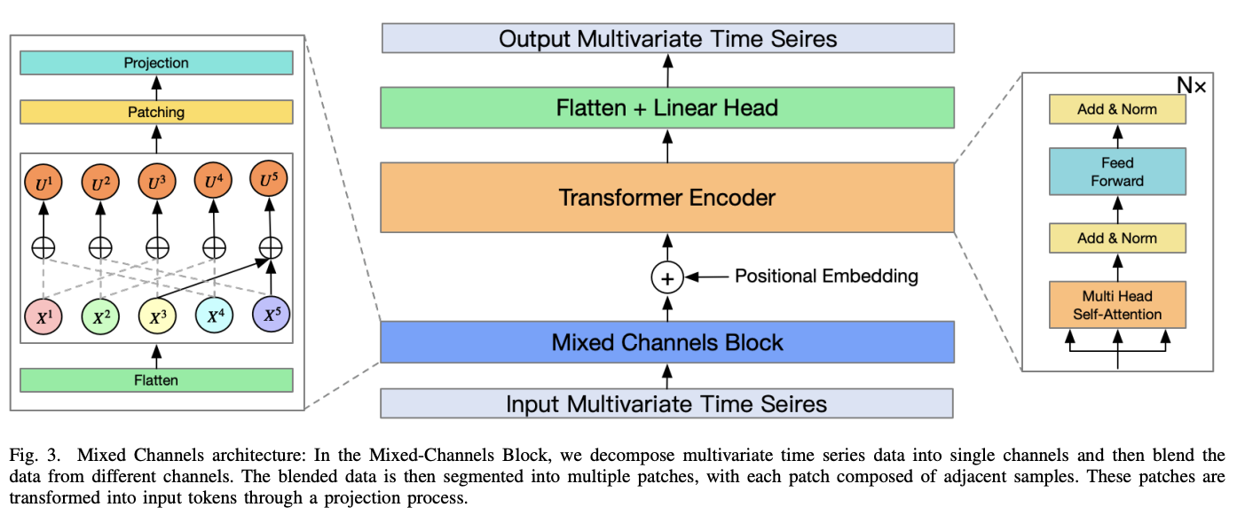
(3) Mixed-Channels Block

a) Flatten

Channel Independent (CI) strategy to flatten

\(X_F=\) Flatten \((X) \in \mathbb{R}^{t M \times 1}\).

• Treated as if it were \(M\) individual samples.

b) Mixed Channels

Combining data from different channels

Procedure

• Step 1) Compute Interval Size \(\left\lfloor\frac{M}{m}\right\rfloor\)

  • where \(m\) is the number of channels to be mixed.

• Step 2) Mixed Channels Operation:

  • For a given time step \(t\),

    starting from the target channel,

    stack every other channel at an interval stride to form \(U^i \in \mathbb{R}^{t \times m}\).

\(\begin{aligned} U^i & =\text { MixedChannels }\left(\mathbf{x}^i, m\right) \\ & =\left[\operatorname{stack}\left(\mathbf{x}^i, C^1, C^2, \ldots, C^m\right)\right] \end{aligned}\).

• where \(C^i\) represents the \(i\)-th channel taken at the \(i\)-th interval,
  • and \(1 \leq i \leq m\).

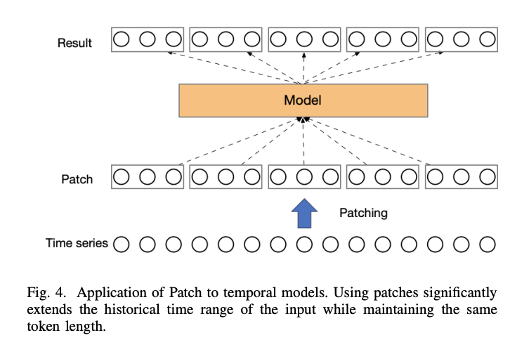
c) Patch and Projection

\(\mathcal{P}^i=\operatorname{Projection}\left(\operatorname{Patch}\left(U^i\right)\right)\).

• \(\mathcal{P}^i \in \mathbb{R}^{P \times N}\),
  • \(P\) : length after projection
  • \(N\) : number of patches
    • \(N=\left\lfloor\frac{(L-p)}{S}\right\rfloor+2\),
    • \(p\) : patch length
    • \(S\): stride

Details

• [Patching] To aggregate the sequence after mixing channels
• [Projection] Single-layer MLP to project channel dependencies as well as adjacent temporal dependencies.

(4) Encoder

native Transformer encoder

• does not explicitly model the sequence’s order

\(\rightarrow\) Learnable additive positional encoding \(\mathcal{W}_{\text {pos }} \in \mathbb{R}^{P \times N}\).

\(\mathcal{X}_{i n}^i=\mathcal{P}^i+\mathcal{W}_{\text {pos }}\).

pass

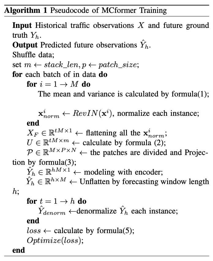
(5) Pseudocode