Retrieval-Augmented Diffusion Models for Time Series Forecasting

Retrieval-Augmented Diffusion Models for Time Series Forecasting

Contents

1. Abstract
2. Introduction
3. Related Work
4. Preliminary
5. Method
6. Experiments

0. Abstract

Factors limiting TS Diffusion

• (1) Insufficient TS datasets
• (2) Absence of guidance

RATD (Retrieval Augmented Time series Diffusion model )

Consists of 2 pars

• (1) Embedding-based retrieval process
• (2) Reference-guided diffusion model

(1) Embedding-based retrieval process

• Retrieves the TS that are most relevant to historical TS from the database as references.

(2) Reference-guided diffusion model

• Uses the references to guide the denoising process

1. Introduction

TS forecasting tasks = Conditional generation tasks

Conditional generative models: learn \(P\left(\boldsymbol{x}^P \mid \boldsymbol{x}^H\right)\)

• Current SOTA: Diffusion models

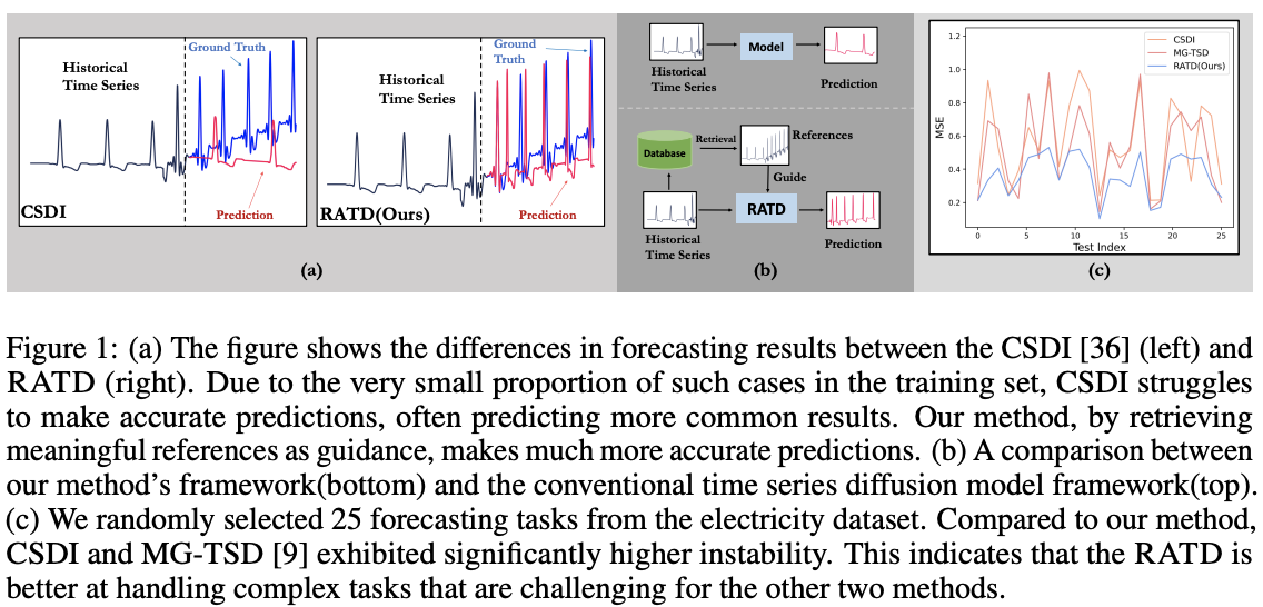
Limitation of TS Diffusion

• Remains unstable in certain scenarios ( Figure 1.c )

• Why?

  • (1) Most TS lack direct semantic or label correspondences

    \(\rightarrow\) Lack meaningful guidance during the generation (reverse)

  • (2) Two shortcomings of the TS datasets

    • 2-1) Insufficient
    • 2-2) Imbalanced

Propose RATD (Retrieval Augmented Time series Diffusion model )

Contributions

• (1) Propose Retrieval Augmented Time series Diffusion (RATD)
  • Utilization of the dataset and providing meaningful guidance in the denoising process.
• (2) Propose Reference Modulated Attention (RMA) module
  • To provide reasonable guidance from the reference
  • w/o introducing excessive additional computational costs
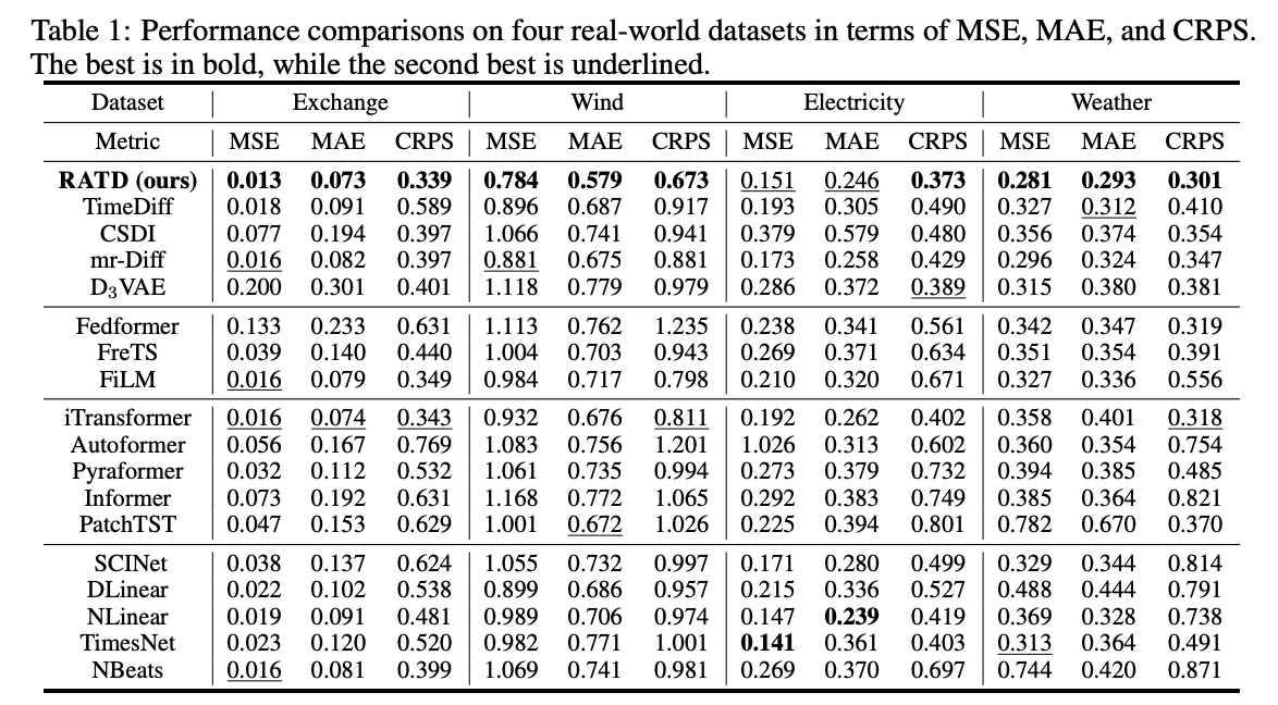
• (3) Experiments on five real-world datasets

2. Related Work

(1) TS Diffusion

TimeGrad [28]

• Conditional diffusion model was first employed
  • Autoregressive approach
  • Denoising process guided by the hidden state

CSDI [36]

• Non-autoregressive generation strategy

SSSD [1]

• Replaced the noise-matching network with a SSSM

TimeDiff [30]

• Incorporated future mix-up and autoregressive initialization into a non-autoregressive framework

MG-TSD [9]

• Utilized a multi-scale generation strategy
• To sequentially predict the main components and details of the TS.

mr-diff [31]

• Utilized diffusion models to separately predict the trend and seasonal components of TS

\(\rightarrow\) Often perform poorly in challenging prediction tasks.

(2) RAG (Retrieval Augmented Generation)

RAG:

• One of the classic mechanisms for generative models.

• Incorporating explicit retrieval steps into NN

NLP & CV domain

[NLP] Leverage retrieval augmentation mechanisms to enhance the quality of language generation

[CV] Focus on utilizing samples from the database to generate more realistic images

TS domain

a) [3]

• Employed memorized similarity information from training data for retrieval

b) MQ-ReTCNN [40]

• Specifically designed for complex TS forecasting tasks involving multiple entities and variables.

c) ReTime [13]

• Creates a relation graph based on the temporal closeness between sequences
• Employs relational retrieval instead of content-based retrieval.

The proposed method still holds significant advantages compared to a)–c).

= References can repeatedly influence the generation

\(\rightarrow\) Allowing references to exert a stronger influence on the entire conditional generation process.

3. Preliminary

Notation

• ” \(s\) “ =Time step
• ” \(t\) “ = Step in the diffusion process.

Generative TS Forecasting

Notation

• Historical TS: \(\boldsymbol{x}^H=\) \(\left\{s_1, s_2, \cdots, s_l \mid s_i \in \mathbb{R}^d\right\}\),
• Target: \(\boldsymbol{x}^P = \left\{s_{l+1}, s_{l+2}, \cdots, s_{l+h} \mid s_{l+i} \in \mathbb{R}^{d^{\prime}}\right\}\left(d^{\prime} \leq d\right)\)

Learn a density \(p_\theta\left(\boldsymbol{x}^P \mid \boldsymbol{x}^H\right)\) that best approximates \(p\left(\boldsymbol{x}^P \mid \boldsymbol{x}^H\right)\),

• \(\min _{p_\theta} D\left(p_\theta\left(\boldsymbol{x}^P \mid \boldsymbol{x}^H\right) \mid \mid p\left(\boldsymbol{x}^P \mid \boldsymbol{x}^H\right)\right),\).

Full TS: \(\left\{s_1, s_2, \cdots, s_{n+h}\right\}=\left[\boldsymbol{x}^H, \boldsymbol{x}^P\right]\).

Conditional TS Diffusion Models

Forward process:

\(\begin{aligned} q\left(\boldsymbol{x}_t \mid \boldsymbol{x}_{t-1}\right) & :=\mathcal{N}\left(\boldsymbol{x}_t ; \sqrt{1-\beta_t} \boldsymbol{x}_{t-1}, \boldsymbol{x}^H, \beta_t \boldsymbol{I}\right) \\ q\left(\boldsymbol{x}_t \mid \boldsymbol{x}_0\right) & :=\mathcal{N}\left(\boldsymbol{x}_t ; \sqrt{\bar{\alpha}_t} \boldsymbol{x}_0, \boldsymbol{x}^H,\left(1-\bar{\alpha}_t\right) \boldsymbol{I}\right) \end{aligned}\).

Reverse process:

\(p_\theta\left(\boldsymbol{x}_{t-1} \mid \boldsymbol{x}_t, \boldsymbol{x}^H\right):=\mathcal{N}\left(\boldsymbol{x}_{t-1} ; \mu_\theta\left(\boldsymbol{x}_t\right), \Sigma_\theta\left(\boldsymbol{x}_t\right), \boldsymbol{x}^H\right)\).

Loss function:

\(\mathcal{L}\left(\boldsymbol{x}_0\right)=\sum_{t=1}^T \underset{q\left(\boldsymbol{x}_t \mid \mid \boldsymbol{x}_0 \mid \mid \boldsymbol{x}^H\right)}{\mathbb{E}} \mid \mid \mu_\theta\left(\boldsymbol{x}_t, t \mid \boldsymbol{x}^H\right)-\hat{\mu}\left(\boldsymbol{x}_t, \boldsymbol{x}_0 \mid \boldsymbol{x}^H\right) \mid \mid ^2\).

4. Method

(1) Overview

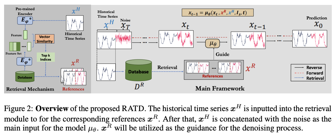
(2) Constructing Retrievl DB for TS

Strategy for constructing DB

Use two different definitions of DB

Definition (1) Entire training set

• \(\mathcal{D}^{\mathcal{R}}:=\left\{\boldsymbol{x}_i \mid \forall \boldsymbol{x}_i \in \mathcal{D}^{\text {train }}\right\}\).
  • where \(\boldsymbol{x}_i=\left\{s_i, \cdots, s_{i+l+h}\right\}\)

Definition (2) Subset containing samples from all categories

• \(\mathcal{D}^{R^{\prime}}=\left\{\boldsymbol{x}_i^c, \cdots, \boldsymbol{x}_q^c \mid \forall c \in \mathcal{C}\right\}\).
  • where \(x_i^k\) is the \(i\)-th sample in the \(k\)-th class of the training set
  • \(\mathcal{C}\) is the category set of the original dataset

For brevity, we represent both databases as \(\mathcal{D}^R\).

(3) Retrieval-Augmented Time Series Diffusion

a) Embedding-Based Retrieval Mechanism

Ideal references \(\left\{s_i, \cdots, s_{i+h}\right\}\)

= Samples where preceding \(n\) points \(\left\{s_{i-n}, \cdots, s_{i-1}\right\}\) is most relevant to the historical TS \(\left\{s_j, \cdots, s_{j+n}\right\}\) in the \(\mathcal{D}^R\).

Quantify the reference between TS using the distance between their embeddings

• Pre-trained encoders \(E_\phi\) a
  • Trained on representation learning tasks
  • Parameter set \(\phi\) is frozen
• \(\mathcal{D}_{\mathrm{emb}}^R=\left\{\left\{i, E_\phi\left(\boldsymbol{x}_{[0: n]}^i\right), \boldsymbol{x}_{[n: n+h]}^i\right\} \mid \forall \boldsymbol{x}^i \in \mathcal{D}^R\right\}\).
  • where \([p: q]\) refers to the subsequence formed by the \(p\)-th point to the \(q\)-th point in the TS
• \(\boldsymbol{v}^H=E_\phi\left(\boldsymbol{x}^H\right)\).

Distance between

• (1) \(\boldsymbol{v}^H\)
• (2) all embeddings in \(\mathcal{D}_{\text {emb }}^R\)

Retrieve the references corresponding to the \(k\) smallest distances.

\(\begin{aligned} & \operatorname{index}\left(\boldsymbol{v}^H\right)=\underset{\boldsymbol{x}^i \in \mathcal{D}_{\text {emb }}^R}{\arg \min } \mid \mid \boldsymbol{v}^H-E_\phi\left(\boldsymbol{x}_{[0: n]}^i\right) \mid \mid ^2 \\ & \boldsymbol{x}^R=\left\{\boldsymbol{x}_{[n: n+h]}^j \mid \forall j \in \operatorname{index}\left(\boldsymbol{v}^H\right)\right\} \end{aligned}\).

We obtain a subset \(\boldsymbol{x}^R\) of \(\mathcal{D}^R\) based on a query \(\boldsymbol{x}^H\),

\(\zeta_k: \boldsymbol{x}^H, \mathcal{D}^R \rightarrow \boldsymbol{x}^R\), where \(\mid \mid \boldsymbol{x}^R \mid \mid =k\).

b) Reference-Guided TS Diffusion Model

Reverse process

• Infer the posterior distribution \(p\left(\boldsymbol{z}^{t a r} \mid \boldsymbol{z}^c\right)\)

\(p\left(\boldsymbol{x} \mid \boldsymbol{x}^H\right)=\int p\left(\boldsymbol{x}_T \mid \boldsymbol{x}^H\right) \prod_{t=1}^T p_\theta\left(\boldsymbol{x}_{t-1} \mid \boldsymbol{x}_t, \boldsymbol{x}^H, \boldsymbol{x}^R\right) \mathcal{D} \boldsymbol{x}_{1: T},\).

• where \(p\left(\boldsymbol{x}_T \mid \boldsymbol{x}^H\right) \approx \mathcal{N}\left(\boldsymbol{x}_T \mid \boldsymbol{x}^H, \boldsymbol{I}\right), p_\theta\left(\boldsymbol{x}_{t-1} \mid \boldsymbol{x}_t, \boldsymbol{x}^H, \boldsymbol{x}^R\right)\)
• Assumption: \(p_\theta\left(\boldsymbol{x}_{t-1} \mid \boldsymbol{x}_t, \boldsymbol{x}\right)=\mathcal{N}\left(\boldsymbol{x}_{t-1} ; \mu_\theta\left(\boldsymbol{x}_t, \boldsymbol{x}^H, \boldsymbol{x}^R, t\right), \Sigma_\theta\left(\boldsymbol{x}_t, \boldsymbol{x}^H, \boldsymbol{x}^R, t\right)\right)\).

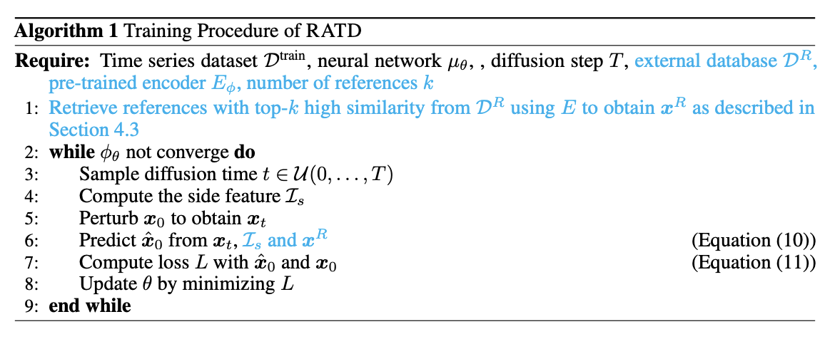
c) Training Procedure

Loss at time step \(t-1\) :

\(\begin{aligned} L_{t-1}^{(x)} & =\frac{1}{2 \tilde{\beta}_t^2} \mid \mid \mu_\theta\left(\boldsymbol{x}_t, \hat{\boldsymbol{x}}_0\right)-\hat{\mu}\left(\boldsymbol{x}_t, \hat{\boldsymbol{x}}_0\right) \mid \mid ^2 \\ & =\gamma_t \mid \mid \boldsymbol{x}_0-\hat{\boldsymbol{x}}_0 \mid \mid \end{aligned}\).

• where \(\hat{\boldsymbol{x}}_0\) are predicted from \(\boldsymbol{x}_t\),
• and \(\gamma_t=\frac{\bar{\alpha}_{t-1} \beta_t^2}{2 \tilde{\beta}_t^2\left(1-\bar{\alpha}_t\right)^2}\)

5. Experiments