ROSE; Register Assisted General Time Series Forecasting with Decomposed Frequency Learning

ROSE: Register Assisted General Time Series Forecasting with Decomposed Frequency Learning

Contents

1. Abstract
2. Introduction
3. Relataed Works
   1. TS Forecasting
   2. TS Pre-training
4. Methodology
   1. Architecture
   2. Decomposed Frequency Learning
   3. Time series register
   4. Training
5. Experiments

0. Abstract

General TS forecasting models

• pre-trained on a large number of TS datasets

Two challenges:

• (1) How to obtain unified representations from multi-domian TS data
• (2) How to capture domain specific features from TS data

ROSE

Register Assisted General Time Series Forecasting Model with Decomposed Frequency Learning

• Novel pre-trained model for TS forecasting

• Pretraining task: Decomposed Frequency Learning

  • decomposes coupled semantic and periodic information in TS

    ( with frequency-based masking and reconstruction )

• Time Series Register

  • learns to generate a register codebook

    • to capture “domain-specific” representations during pretraining

  • enhances “domain-adaptive” transfer

    • by selecting related register tokens on downstream tasks

  • SOTA forecasting performance on 8 real-world benchmarks

    ( + few-shot scenarios )

1. Introduction

Challengs of applying general TS model to heterogeneous TS data

• (1) Obtaining a unified representation
• (2) Adaptive transferring information from multi-domain TS to specific downstream scenarios

(1) Obtaining a UNIFIED representation

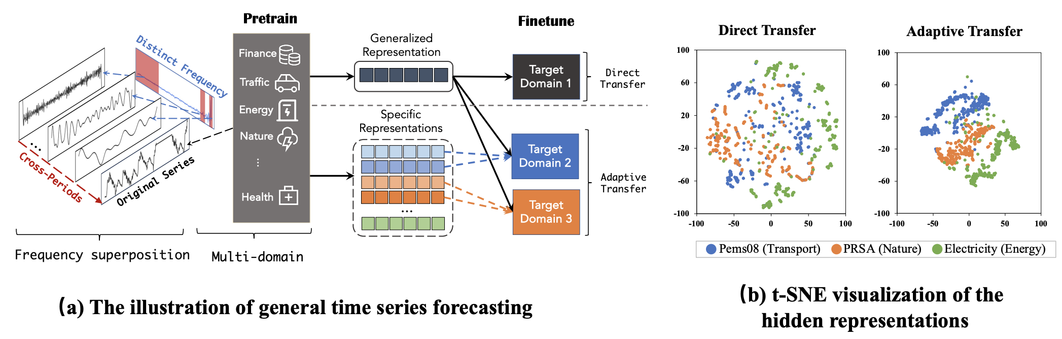
• TS from each domain = multiple frequency components ( = frequency superposition )
• Frequency superposition
  • leads to coupled semantic and periodic information in the time domain.
• Large-scale TS data from different domains
  • complex temporal patterns and frequency diversity

(2) ADAPTIVE transferring information from multi-domain TS

• Multi-source TS data originate from various domains

  • exhibit domain-specific information

• Existing time series pre-training frameworks

  • focus mainly on capturing generalized features during pre-training
  • overlook domain-specific features

  \(\rightarrow\) Necessary to learn domain-specific information during pre-training and adaptively transfer the specific representations to each target domain ( = adaptive transfer )

Two difficulties of adaptive transfer

• (a) Capturing domain-specific information in pre-training
• (b) Adaptive use of domain-specific information in various downstream tasks

ROSE

(1) Decomposed Frequency Learning

• Learns generalized representations to solve the issue with coupled semantic and periodic information.
• Step 1) Decomposition with Fourier transform
  • With a novel frequency-based mask method

• Step 2) Convert it back to the time domain

  • Obtain decoupled TS for reconstruction.

  \(\rightarrow\) Disentanglement … benefit the model to learn generalized representations

(2) Time Series Register (TS-Register)

• Learns domain-specific information in multi-domain data
• Register codebook
  • [Pretraining] Generate register tokens to learn each domain-specific information
  • [Downstream] Adaptively selects vectors from the register codebook that are close to the target domain of interest.
• During fine-tuning, we incorporate learnable vectors into the selected register tokens to complement target specific information to perform more flexible adaptive transfer.

Contribution

1. ROSE = Novel general TS forecasting model
   • using multi-domain datasets for pre-training
   • improve downstream fine-tuning performance and efficiency.

2. Propose a novel Decomposed Frequency Learning

   • employs multi-frequency masking to decouple complex temporal patterns

     \(\rightarrow\) empowers the model’s generalization capability

3. Propose TS-Register
   • (pre-training) to capture domain-specific information
   • (fine-tuning) enables adaptive transfer of target-oriented specific information for downstream tasks
4. Our experiments with 8 real-world benchmarks

2. Related Works

(1) TS forecasting

pass

(2) TS pre-training

Multi-source TS pre-training

• MOMENT [31] and MOIRAI [8]
  • adopt a BERT-style pre-training approach
• Timer [2] and PreDcT [32]
  • use a GPT-style pre-training approach, giving rise to improved performance in TS prediction.

\(\rightarrow\) Above methods overlook domain-specific information from multisource data

ROSE

• Pre-trains on large-scale data from various domains

• Considers both generalized representations and domain-specific information

  \(\rightarrow\) Facilitates flexible adaptive transfer in downstream tasks

3. Methodology

Problem Definition

Multivariate TS: \(\mathbf{X}_t=\left\{\mathbf{x}_{t-L: t}^i\right\}_{i=1}^C\), where \(\mathbf{x}_{t-L: t}^i \in \mathbb{R}^L\)

• \(L\) : look-back window
• \(C\) : number of channels

Forecasting task

• Predict the future values \(\hat{\mathbf{Y}}_t=\left\{\hat{\mathbf{x}}_{t: t+F}^i\right\}_{i=1}^C\),
  • \(F\): forecast horizon
• \(\mathbf{Y}_t=\left\{\mathbf{x}_{t: t+F}^i\right\}_{i=1}^C\) : ground truth

General TS forecasting model

• [Pre-train] with multi-source datasets \(\mathbf{D}_{\text {pre-train }}=\) \(\left\{\left(\mathbf{X}_t^j, \mathbf{Y}_t^j\right)\right\}_{j=1}^N\),
  • where \(N\) is the number of datasets.
• [Downstream task]
  • fine-tuned with a training dataset \(\mathbf{D}_{\text {train }}=\left\{\left(\mathbf{X}_t^{\text {train }}, \mathbf{Y}_t^{\text {train }}\right)\right\}\)
  • tested with \(\mathbf{D}_{\text {test }}=\left\{\left(\mathbf{X}_t^{\text {test }}, \mathbf{Y}_t^{\text {test }}\right)\right\}\) to predict \(\hat{\mathbf{Y}}_t^{\text {test }}\),
• where \(\mathbf{D}_{\text {pre-train }}, \mathbf{D}_{\text {train }}\) and \(\mathbf{D}_{\text {test }}\) are pairwise disjoint.

( + Alternatively, the model could be directly tested using \(\mathbf{D}_{\text {test }}\) without fine-tuning with \(\mathbf{D}_{\text {train }}\) to predict \(\hat{\mathbf{Y}}_t^{\text {test }}\) )

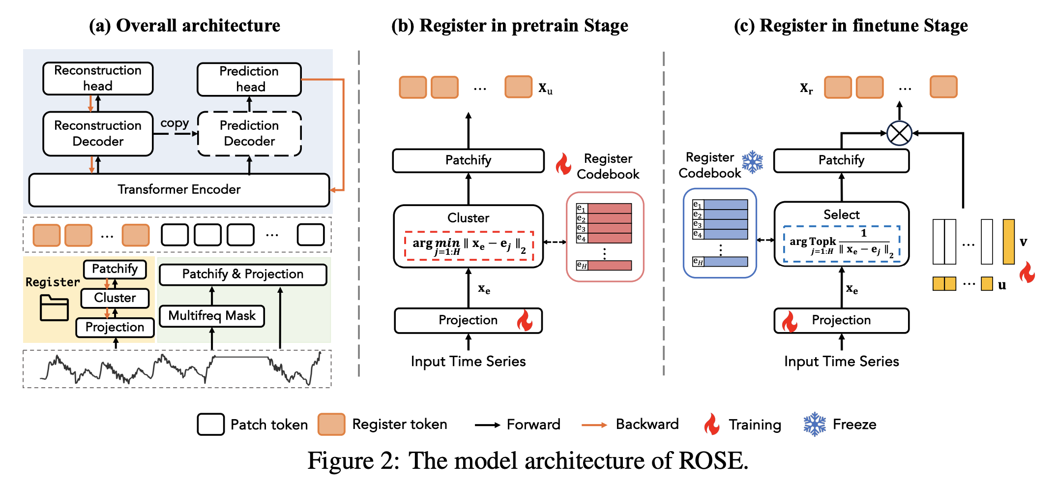
(1) Architecture

TS forecasting paradigm of ROSE contains two steps

• (1) Pre-training
  • pre-trained on large-scale datasets from various domains, with
    • 1-1) Reconstruction
    • 1-2) Prediction
• (2) Fine-tuning
  • fine-tunes with a target dataset in the downstream scenario

• Encoder-Decoder architecture
• Backbone = Transformer
  • effectively capture temporal dependencies
• Channel-independent (CI)

a) Input Representations

To enhance the generalization of ROSE for adaptive transferring ..

\(\rightarrow\) model the inputs \(\mathbf{x}\) with patch tokens and register tokens

Two tokens

• (1) Patch tokens
  • obtained by partitioning the TS using patching layers
• (2) Register tokens
  • obtained by linear mapping and clustering each of the entire TS input into discrete embedding
  • to capture domain-specific information

(2) Decomposed frequency learning

TS = composed of multiple combined frequency components

• Resulting in overlapping of different temporal variations.
• Low-frequency
  • overall trends and longer-scale variations
• High-frequency
  • information about short-term fluctuations and shorter-scale variations

\(\rightarrow\) Propose decomposed frequency learning

• based on multi-freq masking
• to understand the TS from multiple-frequency perspectives
  • which enhances the model’s ability to learn generalized representations

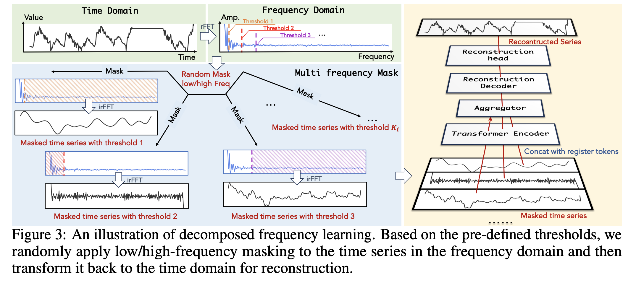
b) Multi-freq masking

\[\mathbf{x}_{\text {freq }}=\operatorname{rFFT}(\mathbf{x})\]

• Input: \(\mathbf{x} \in \mathbb{R}^L\),

• Real Fast Fourier Transform \((\mathrm{rFFT})\)

• Output: \(\mathbf{x}_{\mathrm{freq}} \in \mathbb{R}^{L / 2}\).

To separately model high-frequency and low-frequency information …

Sample …

• \(K_{\mathrm{f}}\) thresholds: \(\tau_1, \tau_2, \tau_3, \ldots, \tau_{K_{\mathrm{f}}}\)
  • where \(\tau \in \operatorname{Uniform}(0, a), a<L / 2\),
• \(K_{\mathrm{f}}\) random numbers: \(\mu_1, \mu_2, \mu_3, \ldots, \mu_{K_{\mathrm{f}}}\)
  • where \(\mu \in \operatorname{Bernoulli}(1, p)\).

for multi-frequency masks

Each pair of \(\tau_i\) and \(\mu_i\) = \(i_{\text {th }}\) frequency mask

\(\rightarrow\) Generates a mask matrix \(\mathbf{M} \in\{0,1\}^{K_{\mathrm{f}} \times L / 2}\),

• Row = \(i_{t h}\) frequency mask
• Column = \(j_{t h}\) frequency
  • mask=0: masked
  • mask=1: unmasked

\(m_{i j}=\left\{\begin{array}{cl} \mu_i & , \text { if } \mathbf{x}_{\mathrm{freq}_j}<\tau_i \\ \left(1-\mu_i\right) & , \text { if } \mathbf{x}_{\mathrm{freq}_j}>\tau_i \end{array},\right.\).

• \(\tau_i\) and \(\mu_i\) : threshold and random number for the \(i_{t h}\) frequency domain mask
• \(\mathbf{x}_{\text {freq }_j}\) : \(j_{t h}\) frequency of \(\mathbf{x}_{\text {freq }}\).
  • If \(\mu_i=1\) … mask HIGH frequency
  • If \(\mu_i=o\) … mask LOW frequency

\(\mathbf{X}_{\text {mask }}=\operatorname{irFFT}\left(\mathbf{X}_{\text {freq }} \odot \mathbf{M}\right)\).

• Step 1) After obtaining the mask matrix \(\mathbf{M}\), ….

• Step 2) Replicate \(\mathbf{x}_{\text {freq }}\) of \(K_{\mathrm{f}}\) times

  \(\rightarrow\) Get the \(\mathbf{X}_{\text {freq }} \in \mathbb{R}^{K_{\mathrm{f}} \times L / 2}\)

• Step 3) Element-wise Hadamard product with the mask matrix \(\mathbf{M}\)

  \(\rightarrow\) Get masked frequency of TS

• Step 4) inverse Real Fast Fourier Transform (irFFT) to convert

  \(\rightarrow\) Get \(K_{\mathrm{f}}\) masked sequences \(\mathbf{X}_{\text {mask }}=\left\{\mathbf{x}_{\text {mask }}^i\right\}_{i=1}^{K_{\mathrm{f}}}\),

  • where each \(\mathbf{x}_{\text {mask }}^i \in \mathbb{R}^L\) corresponding to masking with a different threshold \(\tau_i\).

c) Representation learning

Step Divide each sequence \(\mathbf{x}_{\text {mask }}^i\) into \(P\) non-overlapping patches

• \(\mathbf{x}_{\text {mask }}^i \in \mathbb{R}^L\).

Step 2) Patch Embedding … \(P\) patch tokens ( with linear layer)

\(\rightarrow\) Get \(\mathcal{X}_{\mathrm{mp}}=\left\{\mathbf{X}_{\mathrm{mp}}^i\right\}_{i=1}^{K_{\mathrm{f}}}\) to capture general information

• where \(\mathbf{X}_{\mathrm{mp}}^i \in \mathbb{R}^{P \times D}\)

Step 3) Replicate the register tokens \(\mathbf{X}_{\mathrm{u}}\) of \(K_{\mathrm{f}}\) times

\(\rightarrow\) Get \(\mathcal{X}_{\mathrm{u}} \in \mathbb{R}^{K_{\mathrm{f}} \times N_{\mathrm{r}} \times D}\)

• where \(\mathbf{X}_{\mathrm{u}} \in \mathbb{R}^{N_{\mathrm{r}} \times D}\) is obtained by inputting the original sequence into the TS-Register,

Step 4) Concatenate (a) & (b)

• (a) Patch tokens \(\mathcal{X}_{\mathrm{mp}}\)
• (b) Register tokens \(\mathcal{X}_{\mathrm{u}}\)

Step 5) Transformer encoder

• Representation of each masked series.
• Aggregated to yield a unified representation \(\mathbf{S} \in \mathbb{R}^{\left(N_{\mathrm{r}}+P\right) \times D}\) :

\(\left.\left.\mathbf{S}=\text { Aggregator(Encoder(Concatenate }\left(\mathcal{X}_{\mathrm{mp}}, \mathcal{X}_{\mathrm{u}}\right)\right)\right)\).

d) Reconstruction task

Feed \(\mathbf{S}\) into the reconstruction decoder

Reconstruct the original sequence \(\hat{\mathbf{x}} \in \mathbb{R}^L\)

Note thta frequency domain masking affects the overall TS, we compute the Mean Squared Error (MSE) reconstruction loss for the entire TS

• \(\mathcal{L}_{\text {reconstruction }}= \mid \mid d\mathbf{x}-\hat{\mathbf{x}} \mid \mid d_2^2\).

(3) Time series register

By decomposed frequency learning…

\(\rightarrow\) we can obtain the domain-GENERAL representations

Additionally, propose the TS-Register for domain-SPECIFIC information

TS-Register

• Step 1) Clusters domain-specific information into register tokens
• Step 2) (Pre-training) Stores such domain-specific information in the register codebook
• Step 3) (Fine-tuning) Adaptively selects similar information from the register codebook
  • to enhance the target domain

Details

• Randomly initialized register codebook \(\mathbf{E} \in \mathbb{R}^{H \times D_{\mathrm{r}}}\)
  • with \(H\) cluster center vectors \(\mathbf{e}_i \in \mathbb{R}^{D_{\mathrm{r}}}, i \in\{1,2, \ldots, H\}\).
• Projection: input TS \(\mathbf{x} \in \mathbb{R}^L\) \(\rightarrow\) embedding \(\mathbf{x}_{\mathrm{e}} \in \mathbb{R}^{D_{\mathrm{r}}}\)
  • through a linear layer.

a) Pre-training stage.

• Use the register codebook to cluster these embeddings

  ( which generate domain-specific information )

• Store them in pre-training.
• Find a cluster center vector \(\mathbf{e}_\delta\) from the register codebook \(\mathbf{E}\)
  • \(\delta=\underset{j=1: H}{\arg \min } \mid \mid d\mathbf{x}_{\mathrm{e}}-\mathbf{e}_j \mid \mid d_2\).
• To update the cluster center vectors … loss function:
  • \(\mathcal{L}_{\text {register }}= \mid \mid d\operatorname{sg}\left(\mathbf{x}_{\mathrm{e}}\right)-\mathbf{e}_\delta \mid \mid d_2^2+ \mid \mid d\mathbf{x}_{\mathrm{e}}-\operatorname{sg}\left(\mathbf{e}_\delta\right)\mid \mid d_2^2\).
    • First term = update the register codebook \(\mathbf{E}\),
    • Second term = update the parameters of the linear layer that learns \(\mathbf{x}_{\mathrm{e}}\).

Summary: Vectors in the register codebook \(\mathbf{E}\)

• cluster the embeddings of different data

• learn the domain-specific centers for pre-trained datasets

  ( = represent domain-specific information )

\(\mathbf{X}_{\mathrm{u}} \in \mathbb{R}^{N_{\mathrm{r}} \times D}\) = register tokens

• Cluster center vector \(\mathbf{e}_\delta\) is then patched into register tokens
  • \(N_{\mathrm{r}}\): # of the register tokens
• Used as the prefix of the patch tokens \(\mathbf{X}_{\mathrm{p}} \in \mathbb{R}^{P \times D}\)
  • provide domain-specific information.

b) Fine-tuning stage

Freeze the register parameters

• to adaptively use this domain-specific information

top-k strategy

• Selects top-k similar vectors in the register codebook
• Uses their average as \(\overline{\mathbf{e}}_k\)
  • \(\rightarrow\) also patched into \(\mathbf{X}_{\mathrm{d}} \in \mathbb{R}^{N_{\mathrm{r}} \times D}\)

\(\overline{\mathbf{e}}_k=\frac{1}{k} \sum_{i=1}^k \mathbf{e}_{\delta_i},\{\delta_1, \cdots, \delta_k\}=\underset{j=1: H}{\arg \operatorname{Topk}}(\frac{1}{\mid \mid d\mathbf{x}_{\mathrm{e}}-\mathbf{e}_j \mid \mid d_2}) .\).

Additionally set a matrix \(\mathbf{A} \in \mathbb{R}^{N_{\mathrm{r}} \times D}\) to adjust \(\mathbf{X}_{\mathrm{d}}\)

\(\rightarrow\) to complement the specific information of downstream data.

\(\mathbf{A}\) is set as a low-rank matrix:

• \(\mathbf{A}=\mathbf{u} \times \mathbf{v}^{\mathrm{T}}\).
  • where \(\mathbf{u} \in \mathbb{R}^{N_{\mathrm{r}}}\) and \(\mathbf{v} \in \mathbb{R}^D\),
• only the vectors \(\mathbf{u}\) and \(\mathbf{v}\) need to be retrained in the fine-tuning step

Register token \(\mathbf{X}_{\mathrm{r}}\) of the downstream scenario

• \(\mathbf{X}_{\mathrm{r}}=\mathbf{X}_{\mathrm{d}} \odot \mathbf{A}\).
  • \(\mathbf{X}_{\mathrm{d}}\) = domain-specific information obtained at the pre-train stage
  • \(\mathbf{A}\) = downstream dataset-specific information.

(4) Training

Co-train ..

• (1) Supervised prediction
• (2) Self-supervised reconstruction

Why (1)?

• Uses multi-frequency mask to learn unified features that are more applicable to the downstream prediction task.

a) Prediction task (SL)

Notation

• Input TS: \(\mathbf{x} \in \mathbb{R}^L\)
• Spliced Input TS & Mapped : \(\mathbf{X}_{\mathrm{p}} \in \mathbb{R}^{P \times D}\)

Four prediction heads

• mapping to prediction lengths of \(\{96,192,336,720\}\)

Concatenation

• (1) Patch tokens \(\mathbf{X}_{\mathrm{p}}\)
• (2) Register tokens \(\mathbf{X}_{\mathrm{u}}\)

\(\rightarrow\) [(1), (2)] Feed into the transformer encoder, prediction decoder, and prediction heads to obtain four prediction results \(\hat{\mathbf{Y}}_F\), where \(F \in\) \(\{96,192,336,720\}\).

\(\mathcal{L}_{\text {prediction }}=\sum_{F \in\{96,192,336,720\}} \mid \mid d\mathbf{Y}_F-\hat{\mathbf{Y}}_F \mid \mid d_2^2\).

b) Pre-training

Learns generalized features

\(\rightarrow\) Parameters of the reconstruction decoder are copied to the prediction decoder

( To avoid prediction training affecting the generalization performance of the model, the gradients of the prediction heads are skipped at back-propagation )

Overall pre-training loss

\(\mathcal{L}_{\text {pre-train }}=\mathcal{L}_{\text {reconstruction }}+\mathcal{L}_{\text {prediction }}+\mathcal{L}_{\text {register }}\).

c) Fine-tuning

pass

4. Experiments

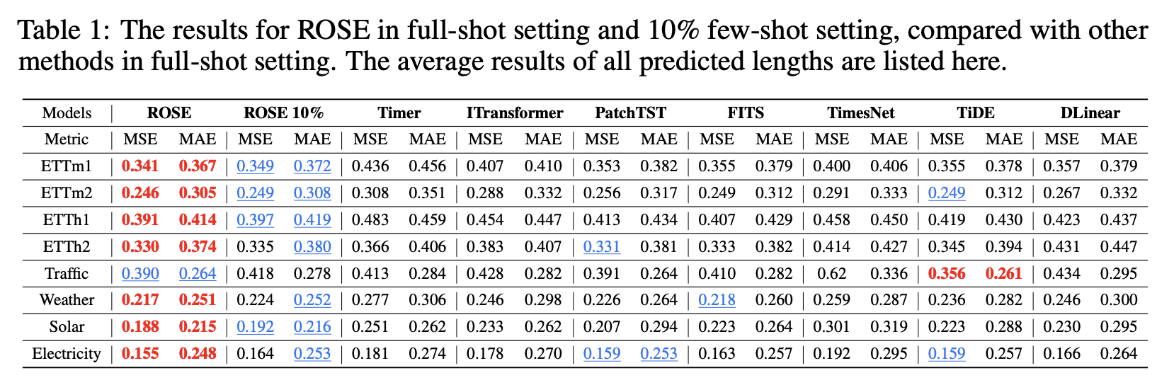
(1) Main Results

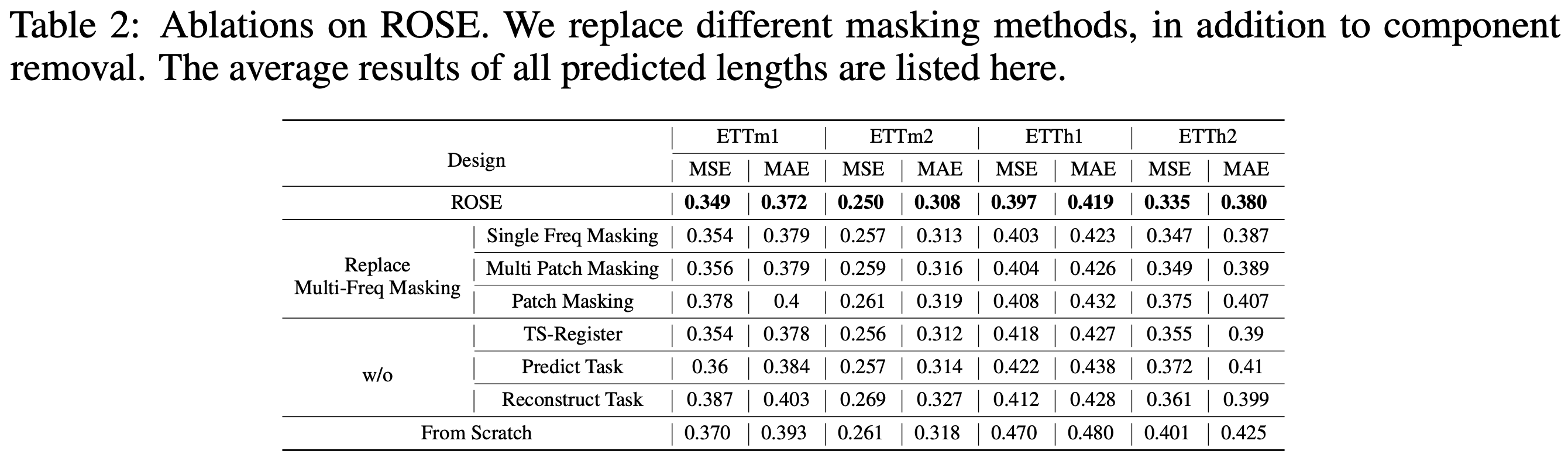
(2) Ablation studies

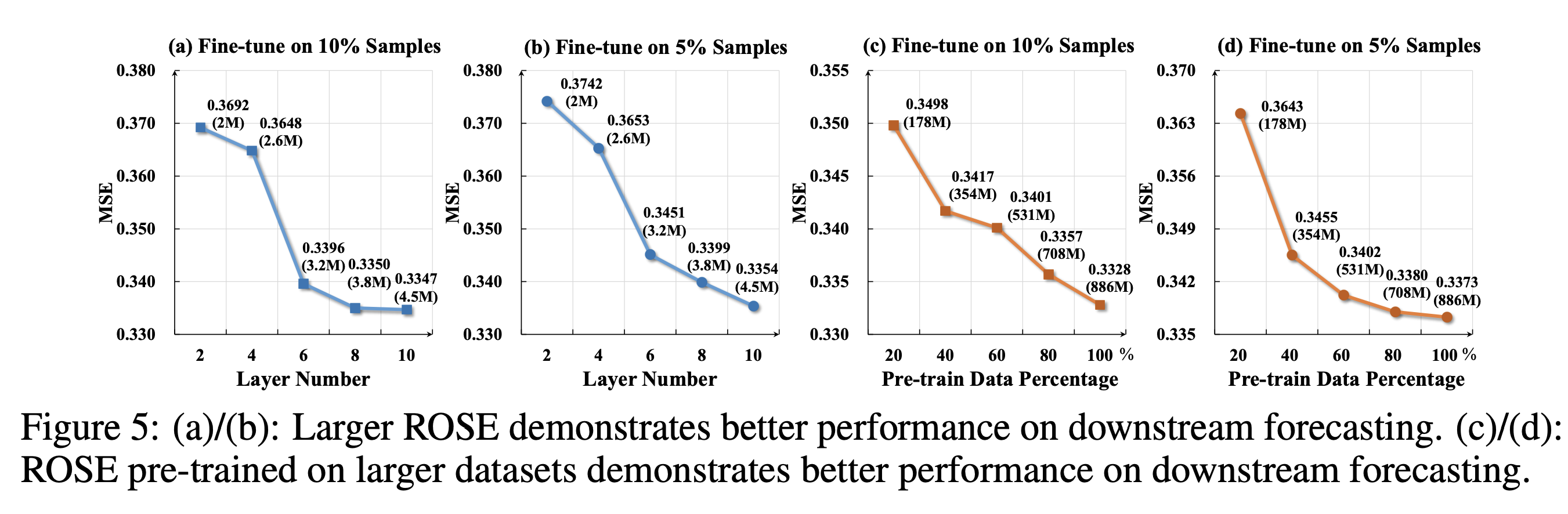
(3) Scalability

(4) Model Analysis

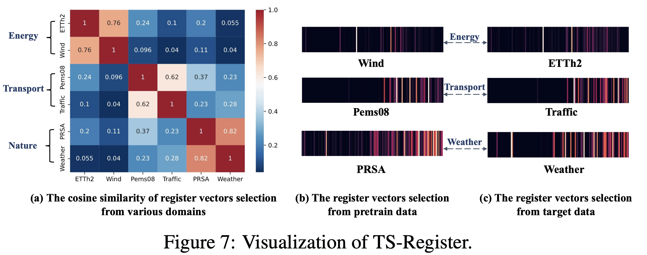
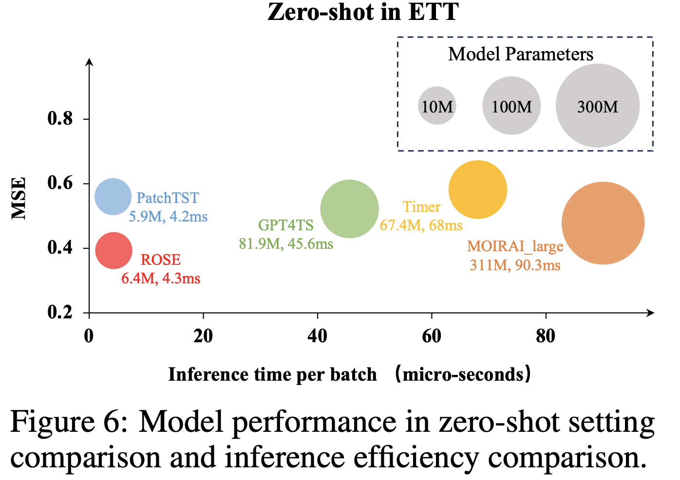
a) Zero-shot & Inference efficiency

b) Visuaalization of TS-Register