TimeMixer++; A General TS Pattern Machine for Universal Predictive Analysis

TimeMixer++; A General TS Pattern Machine for Universal Predictive Analysis

Contents

1. Abstract
2. Introduction
3. Related Work
4. TimeMixer++
   1. Structure overview
   2. Mixer block
5. Experiments
   1. Main Results
   2. Model Analysis

0. Abstract

TS pattern machine (TSPM)

• For a broad range of TS tasks
  • forecasting, classification, anomaly detection, imputation
• Through powerful representation and pattern extraction capabilities.

Traditional TS models

• Struggle to capture universal patterns

  \(\rightarrow\) Limiting their effectiveness across diverse tasks

TimeMixer++

a) Time & Frequency

• (1) Multiple scales in the time domain domain
• (2) Various resolutions in the frequency domain

\(\rightarrow\) Employ various mixing strategies to extract intricate, task-adaptive TS patterns.

b) TimeMixer++

TSPM that processes multi-scale TS using

• (1) Multi-resolution time imaging (MRTI)
• (2) Time image decomposition (TID)
• (3) Multi-scale mixing (MCM)
• (4) Multi-resolution mixing (MRM)

to extract comprehensive temporal patterns.

c) Experiments

SOTA across 8 TS analytical tasks,

surpassing both general-purpose and task-specific models

1. Introduction

TS pattern machines (TSPMs)

• Unified model architecture capable of handling a broad range of TS tasks across domains (Zhou et al., 2023; Wu et al., 2023).

• Key: Ability to recognize and generalize TS patterns

  \(\rightarrow\) Enabling the model to uncover meaningful temporal structures and adapt to varying TS tasks

Traditional works

• (1) RNNs: Struggle to capture long-term dependencies due to limitations like Markovian assumptions and inefficiencies.

• (2) TCNs: Efficiently capture local patterns but face challenges with long-range dependencies (e.g., seasonality and trends) because of their fixed receptive fields.

• (3) Reshape TS into 2D

  • based on frequency domain information (Wu et al., 2023)
  • downsample the time domain (Liu et al., 2022a)

  \(\rightarrow\) Fall short in comprehensively capturing long-range patterns.

• (4) Transformers: Leverage token-wise self-attention to model long-range dependencies

  \(\rightarrow\) Often involve overlapping contexts at a single time point, such as daily, weekly…

  \(\rightarrow\) Difficult to represent TS patterns effectively as tokens

Question: What capabilities must a model possess, and what challenges must it overcome, to function as a TSPM?

Multiscale Nature of TS

Reconsider how TS are generated from continuous real-world processes sampled at various scales.

• ex) Daily data capture hourly fluctuations
• ex) Yearly data reflect long-term trends and seasonal cycles

\(\rightarrow\) This multi-scale, multiperiodicity nature presents a significant challenge for model design, as each scale emphasizes different temporal dynamics

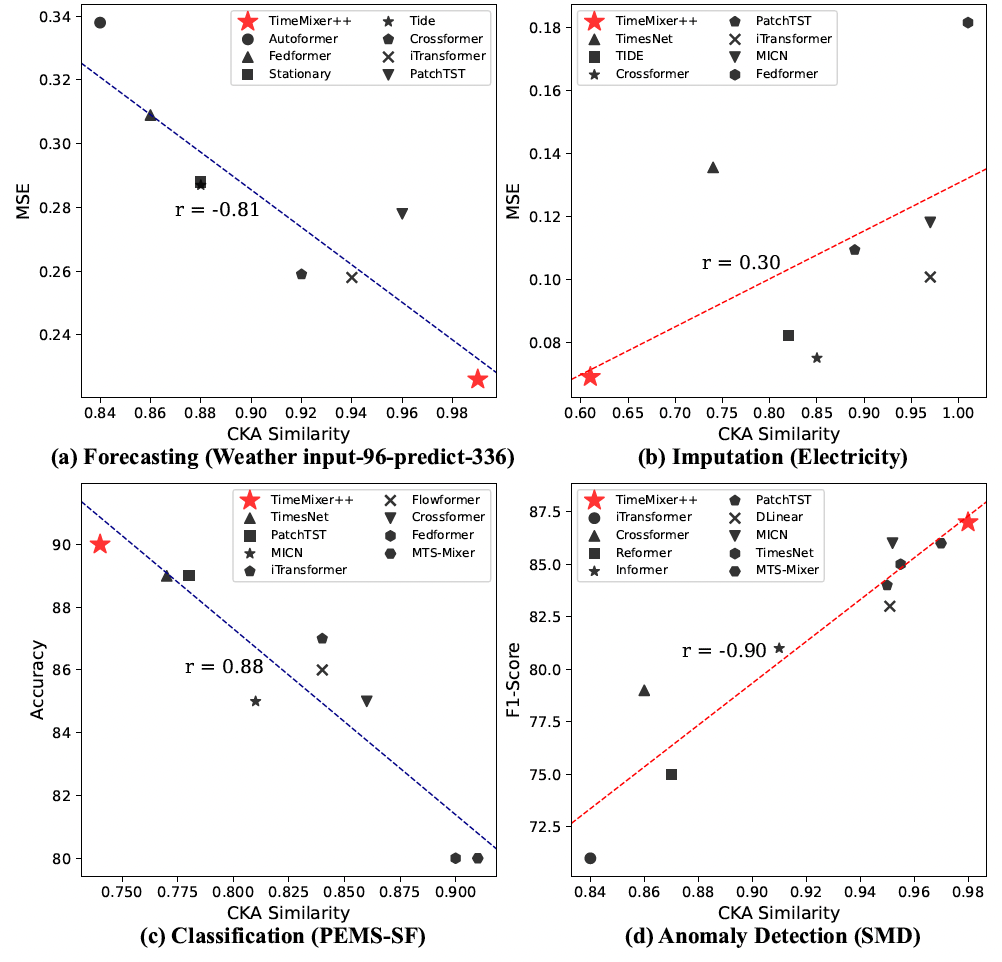
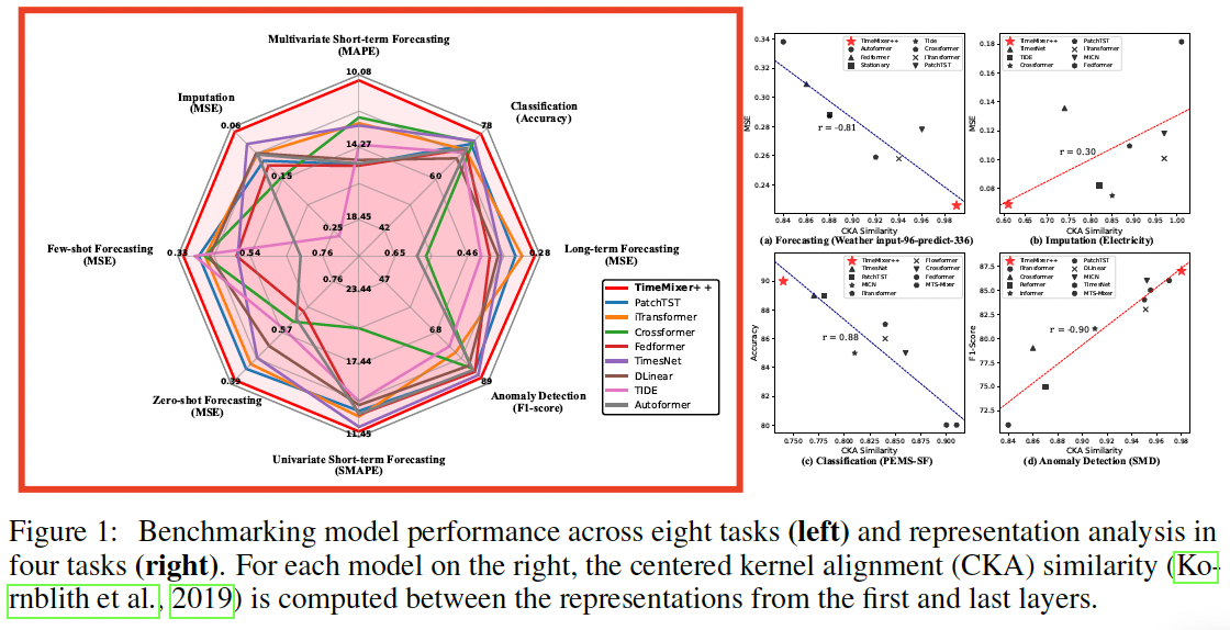
Figure 1) Challenge in constructing a general TSPM

• (a) Lower CKA similarity = More diverse representations across layers

  \(\rightarrow\) Advantageous for tasks like imputation and anomaly detection

  • Require capturing irregular patterns & handling missing data.
  • Diverse representations across layers help manage variations across scales and periodicities.

• (b) Higher CKA similarity = Less diverse representations across layers

  \(\rightarrow\) Advantageous for tasks like forecasting and classification

  • Consistent representations across layers better capture stable trends and periodic patterns

Difference in (a) &. (b)

\(\rightarrow\) Emphasizes the challenge of designing a universal model flexible enough to adapt to multi-scale and multi-periodicity patterns across various analytical tasks, which may favor either diverse or consistent representations

TimeMixer

(1) General purpose TSPM designed to capture (2) general, task-adaptive TS patterns by tackling the complexities of (3) multi-scale and multi-periodicity dynamics

Key idea = Simultaneously capture intricate TS patterns across ..

• a) multiple scales in the time domain
• b) various resolutions in the frequency domain

TSPM that processes multi-scale TS using

• (1) Multi-resolution time imaging (MRTI)
• (2) Time image decomposition (TID)
• (3) Multi-scale mixing (MCM)
• (4) Multi-resolution mixing (MRM)

to extract comprehensive temporal patterns.

Details

• (1) MRTI: Transforms multi-scale TS into multi-resolution time images

  \(\rightarrow\) Capture patterns across both temporal and frequency domains

• (2) TID: Leverages dual-axis attention to extract seasonal and trend patterns
• (3) MCM: Hierarchically aggregates these patterns across scales
• (4) MRM: Adaptively integrates all representations across resolutions

2. Related Work

(1) TS Analysis

Statistical methods

• ARIMA (Anderson & Kendall, 1976) and STL (Cleveland et al., 1990)

  \(\rightarrow\) Effective for periodic and trend patterns but struggle with non-linear dynamics

Deep learning models

• RNNs: Capture sequential dependencies but face limitations with long-term dependencies.
• TCNs: Improve local pattern extraction but are limited in capturing long range dependencies.
• TimesNet (Wu et al., 2023): Enhances long-range pattern extraction by treating TS as 2D signals
• MLPs: Offer simplicity and effectiveness
• Transformer-based models: Self-attention to model long-range dependencies

Given the strengths and limitations discussed above …

\(\rightarrow\) growing need for a TSPM capable of effectively extracting diverse patterns, adapting to various TS analytical tasks, and possessing strong generalization capabilities

(2) Hierarchical TS Modeling

Emphasis on the decomposition!

• Step 1) Use moving averages (MA) to discern seasonal and trend components
• Step 2) Subsequently modeled using ..
  • (1) Attention mechanisms (Wu et al., 2021; Zhou et al., 2022b)
  • (2) Convolutional networks (Wang et al., 2023)
  • (3) Hierarchical MLP layers (Wang et al., 2024).

\(\rightarrow\) These components are individually processed prior to aggregation to yield the final output

Limitation?

Such approaches frequently depend on predefined and rigid operations for the disentanglement of seasonality and trends, thereby constraining their adaptability to complex and dynamic patterns.

TimeMixer ++

• a) Disentangles seasonality and trend directly within the latent space via dual-axis attention

  \(\rightarrow\) Enhancing adaptability to a diverse range of TS patterns and task scenarios.

• b) Adopt a multi-scale, multi-resolution analytical framework

  \(\rightarrow\) Facilitating hierarchical interaction and integration across different scales and resolutions

3. TimeMixer++

Key point = Multi-scale + Multi-periodic

TimeMixer++

• General-purpose TS pattern machine
• Processes multi-scale TS using an encoder-only architecture
• Comprises of three components
  • (1) Input projection
  • (2) Stack of Mixerblocks
  • (3) Output projection

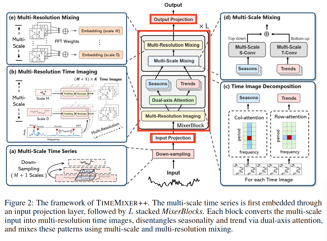
Multi-scale TS

(1) Input TS: \(\mathrm{x}_0 \in \mathbb{R}^{T \times C}\)

(2) Multi-scale representation ( through downsampling )

• (1) Downsampled across \(M\) scales
• (2) With convolution operations with a stride of 2
  • \[\mathrm{x}_m=\operatorname{Conv}\left(\mathrm{x}_{m-1}, \text { stride }=2\right), \quad m \in\{1, \cdots, M\}\]

(3) Result: multi-scale set \(X_{\text {init }}=\left\{\mathrm{x}_0, \cdots, \mathrm{x}_M\right\}\),

• where \(\mathrm{x}_m \in \mathbb{R}^{\frac{\pi}{2} m \mathrm{~J}} \times C\).

(1) Structure Overview

a) Input Projection

CI vs. CD

• (Previous) Channel-independence strategy

  • To avoid projecting multiple variables into indistinguishable channels (Liu et al., 2024a).

• (TimeMixer++) Channel mixing

  • To capture cross-variable interactions

    \(\rightarrow\) Crucial for revealing comprehensive patterns in TS data.

Two components:

• (1) Channel mixing
• (2) Embedding

(1) Channel mixing

• Self-attention to the variate dimensions at the coarsest scale

  • coarsest scale = global context = \(\mathrm{x}_M \in \mathbb{R}^{\left\lfloor\frac{T}{2^M}\right\rfloor \times C}\)

  \(\rightarrow\) Facilitating the more effective integration

• \(\mathbf{x}_M=\text { Channel-Attn }\left(\mathbf{Q}_M, \mathbf{K}_M, \mathbf{V}_M\right)\).

  • variate-wise self-attention
  • \(\mathbf{Q}_M, \mathbf{K}_M, \mathbf{V}_M \in \mathbb{R}^{C \times\left\lfloor\frac{T}{2^T}\right\rfloor}\) are derived from linear projections of \(\mathbf{x}_M\).

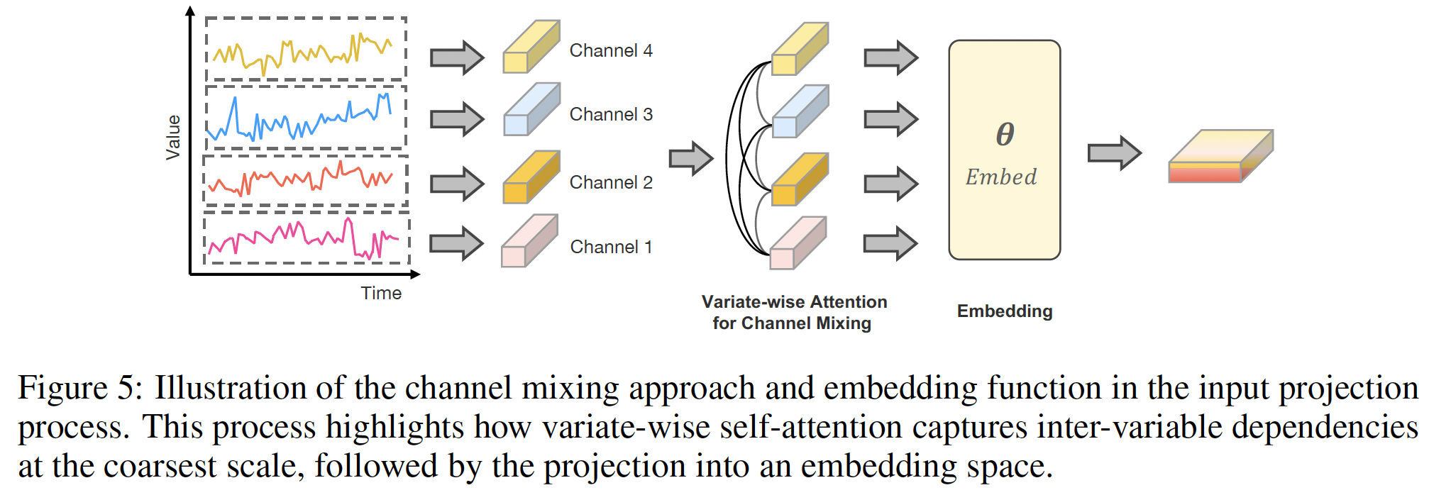
(2) Embedding

• Embed all multi-scale TS into a deep pattern set \(X^0\) using an embedding layer
• Result: \(X^0=\left\{\mathrm{x}_0^0, \cdots, \mathrm{x}_M^0\right\}=\operatorname{Embed}\left(X_{\text {init}}\right)\),
  • where \(\mathrm{x}_m^0 \in \mathbb{R}^{\left\lfloor 2_2^{T-J}\right] \times d_{\text {model}}}\)

b) MixerBlocks

Component: Stack of \(L\) Mixerblocks

\(x^{l+1}=\operatorname{MixerBlock}\left(X^l\right)\),

• where \(X^l=\left\{\mathrm{x}_0^t, \cdots, \mathrm{x}_M^l\right\}\) and \(\mathbf{x}_m^l \in \mathbb{R}^{\left\lfloor\frac{T}{2^m}\right\rfloor \times d_{\text {model }}}\).

Goal: Capture intricate patterns across ..

• Scales in the time domain
• Resolutions in the frequency domain

Process

• (1) Convert multi-scale TS \(\rightarrow\) multi-resolution time images,

• (2) Disentangle seasonal and trend patterns
  • Through time image decomposition
• (3) Aggregate these patterns across different scales and resolutions.

c) Output Projection

After MixerBlocks … obtain the multi-scale representation set \(X^L\).

Note that different scales capture distinct temporal patterns and tasks vary in demands

\(\rightarrow\) Multiple prediction heads

• Each specialized for a specific scale
• Ensemble their outputs!

This design is “task-adaptive”

= Allowing each head to focus on relevant features at its scale, while the ensemble aggregates complementary information to enhance prediction robustness.

\(\text { output }=\operatorname{Ensemble}\left(\left\{\operatorname{Head}_m\left(\mathbf{x}_m^L\right)\right\}_{m=0}^M\right)\).

• Ensemble: averaging / weighted sum …
• Head: linear layer

(2) MixerBlock

Stack in a residual way

• \(x^{l+1}=\text { LayerNorm }\left(x^l+\operatorname{MixerBlock}\left(x^l\right)\right)\).
  • LayerNorm: normalizes patterns across scales and can stabilize the training

TS exhibits complex multi-scale and multi-periodic dynamics

• Multi-resolution analysis (Harti, 1993)
  • Models TS as a composite of various periodic components in the frequency domain
• (Proposal) Multi-resolution time images
  • Converts 1D multi-scale TS into 2D images
  • Based on frequency analysis
  • Goal: Captures intricate patterns across time and frequency domains, enabling efficient use of convolution methods for extracting temporal patterns and enhancing versatility across tasks.

How to process multi-scale TS?

• (1) multi-resolution time imaging (MRTI)
• (2) time image decomposition (TID)
• (3) multi-scale mixing (MCM)
• (4) multi-resolution mixing (MRM)

to uncover comprehensive TS patterns.

a) Multi-Resolution Time Imaging (MRTI)

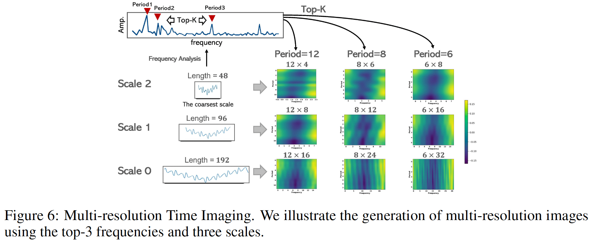
Goal of MRTI: Convert from (a) \(\rightarrow\) (b)

• (a) Input: \(X^l\)
• (b) Output: \((M+1) \times K\) multi-resolution time images via

How? by frequency analysis (Wu et al., 2023)

Identify periods from the coarsest scale \(\mathrm{x}_M^1\)

( = enables global interaction )

Details)

• Apply FFT on \(x_M^t\)
• Select the top- \(K\) frequencies with the highest amplitudes

\(\mathbf{A},\left\{f_1, \cdots, f_K\right\},\left\{p_1, \cdots, p_K\right\}=\operatorname{FFT}\left(\mathbf{x}_M^l\right)\).

• \(\mathbf{A}=\left\{A_{f_1}, \cdots, A_{f_K}\right\}\): unnormalized amplitudes
• \(\left\{f_1, \cdots, f_K\right\}\): Top- \(K\) frequencies
• \(p_k=\left\lceil\frac{T}{f_k}\right\rceil, k \in\{1, \ldots, K\}\) : Corresponding period lengths.

Each 1 D time series \(\mathrm{x}_m^l\) is then reshaped into \(K 2 \mathrm{D}\) images as:

b) Time Image Decomposition

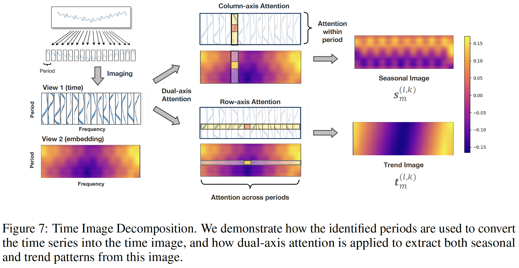
TS patterns: Inherently nested, with overlapping scales and periods.

• e.g.) Weekly sales data: reflects both daily shopping habits and broader seasonal trends

Conventional methods (Wu et al., 2021; Wang et al., 2024)

• Moving averages across the entire TS

\(\rightarrow\) Often blurring distinct patterns.

• Solution: multi-resolution time images

Multi-resolution time images

• Each image \(\mathbf{z}_m^{(l, k)} \in \mathbb{R}^{p_k \times f_{m . k} \times d_{\text {model }}}\) encodes a specific scale and period

  \(\rightarrow\) Enabling finer disentanglement of seasonality and trend

• Apply 2D conv to these images

• Details

  • Columns = TS segments within a period
  • Rows = Consistent time points across periods

  \(\rightarrow\) Facilitates dual-axis attention

• Dual-axis attention

  • (1) Column-axis attention
    • Captures seasonality within periods
  • (2) Row-axis attention
    • Extracts trend across periods

  \(\rightarrow\) Each axis-specific attention focuses on one axis, preserving efficiency by transposing the non-target axis to the batch dimension.

\(\mathbf{s}_m^{(l, k)}=\text { Attention }_{\mathrm{col}}\left(\mathbf{Q}_{\mathrm{col}}, \mathbf{K}_{\mathrm{col}}, \mathbf{V}_{\mathrm{col}}\right)\).

\(\mathbf{t}_m^{(l, k)}=\operatorname{Attention}_{\text {row }}\left(\mathbf{Q}_{\text {row }}, \mathbf{K}_{\text {row }}, \mathbf{V}_{\text {row }}\right)\).

• where \(\mathbf{s}_m^{(l, k)}, \mathbf{t}_m^{(l, k)} \in \mathbb{R}^{p_k \times f_{\mathrm{m} . \mathrm{k}} \times d_{\text {model }}}\) represent the seasonal and trend images

c) Multi-scale Mixing

For each period \(p_k\) …. we obtain

• (1) \(M+1\) seasonal time images
• (2) \(M+1\) trend time images

\(\rightarrow\) \(\left\{\mathbf{s}_m^{(l, k)}\right\}_{m=0}^M\) and \(\left\{\mathbf{t}_m^{(l, k)}\right\}_{m=0}^M\)

Summary of 2D structure

= Allows us to model (1) both seasonal and trend patterns using 2D convolutional layers, which are more (2) efficient and effective at capturing long-term dependencies than traditional linear layers (Wang et al., 2024).

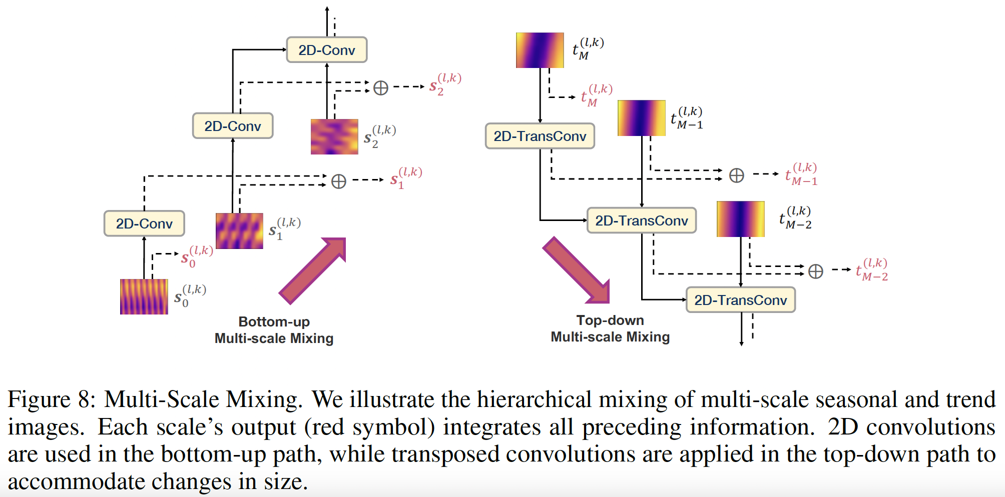
(1) Bottom-up mixing strategy (for seasonal pattern)

• Mix the seasonal patterns from “fine-scale to coarse-scale”
• Why? Longer patterns can be interpreted as compositions of shorter ones
  • (e.g., a yearly rainfall pattern formed by monthly changes)
• \(\text { for } m: 1 \rightarrow M \text { do: } \quad \mathbf{s}_m^{(l, k)}=\mathbf{s}_m^{(l, k)}+2 \mathrm{D}-\operatorname{Conv}\left(\mathbf{s}_{m-1}^{(l, k)}\right)\).
  • 2D-Conv: Composed of two 2D convolutional layers with a temporal stride of 2

(2) Top-down mixing strategy (for trend pattern)

• Mix the trend patterns from “coarse-scale to trend-scale”
• Why? Coarser scales naturally highlight the overall trend.
• \(\text { for } m: M-1 \rightarrow 0 \text{ do} \quad \mathbf{t}_m^{(l, k)}=\mathbf{t}_m^{(l, k)}+2 \mathrm{D}-\operatorname{TransConv}\left(\mathbf{t}_{m+1}^{(l, k)}\right)\),
  • 2D-TransConv: Composed of two 2D transposed convolutional layers with a temporal stride of 2

(3) Aggregation

• Seasonal and trend patterns are aggregated

• How? Summation and reshaped back to a 1D structure
• \(\mathbf{z}_m^{(l, k)}=\underset{2 D \rightarrow 1 D}{\operatorname{Reshape}_{m, k}}\left(\mathbf{s}_m^{(l, k)}+\mathbf{t}_m^{(l, k)}\right), \quad m \in\{0, \cdots, M\}\),
  • where Reshape \({ }_{m, k}(\cdot)\) convert a \(p_k \times f_{m, k}\) image into a time series of length \(p_k \cdot f_{m, k}\).

d) Multi-resolution Mixing

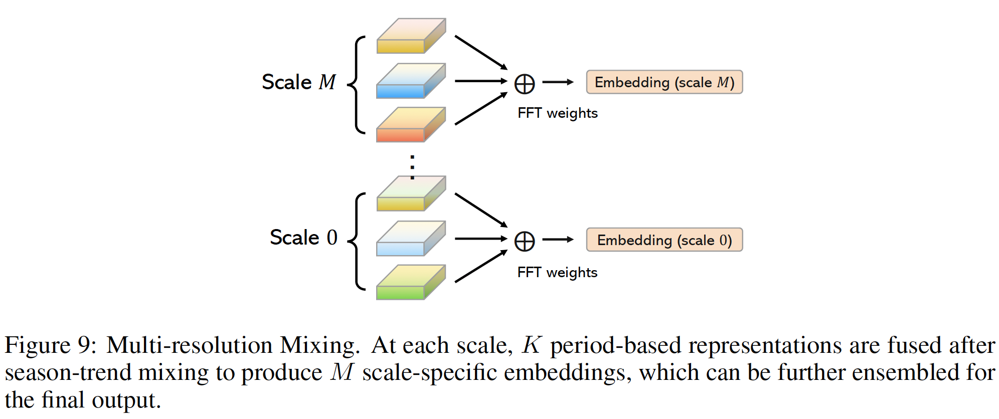
At each scale, we mix the \(K\) periods adaptively!

• Amplitudes \(\mathbf{A}\) = Importance of each period

Aggregate the patterns \(\left\{\mathbf{z}_m^{(l, k)}\right\}_{k=1}^K\) as …

\(\left\{\hat{\mathbf{A}}_{f_k}\right\}_{k=1}^K=\operatorname{Softmax}\left(\left\{\mathbf{A}_{f_k}\right\}_{k=1}^K\right), \quad \mathbf{x}_m^l=\sum_{k=1}^K \hat{\mathbf{A}}_{f_k} \circ \mathbf{z}_m^{(l, k)}, \quad m \in\{0, \cdots, M\}\).

4. Experiments

General time series pattern machine

= extensive experiments across 8 well-established analytical tasks,

• (1) long-term forecasting
• (2) univariate shoft-term forecasting
• (3) multivariate short-term forecasting
• (4) imputation
• (5) classification
• (6) anomaly detection
• (7) few-shot forecasting
• (8) zero-shot forecasting

Summary: Superior performance across 30 well-known benchmarks and against 27 advanced baselines.

(1) Main Results

Task 1: Long-term forecasting

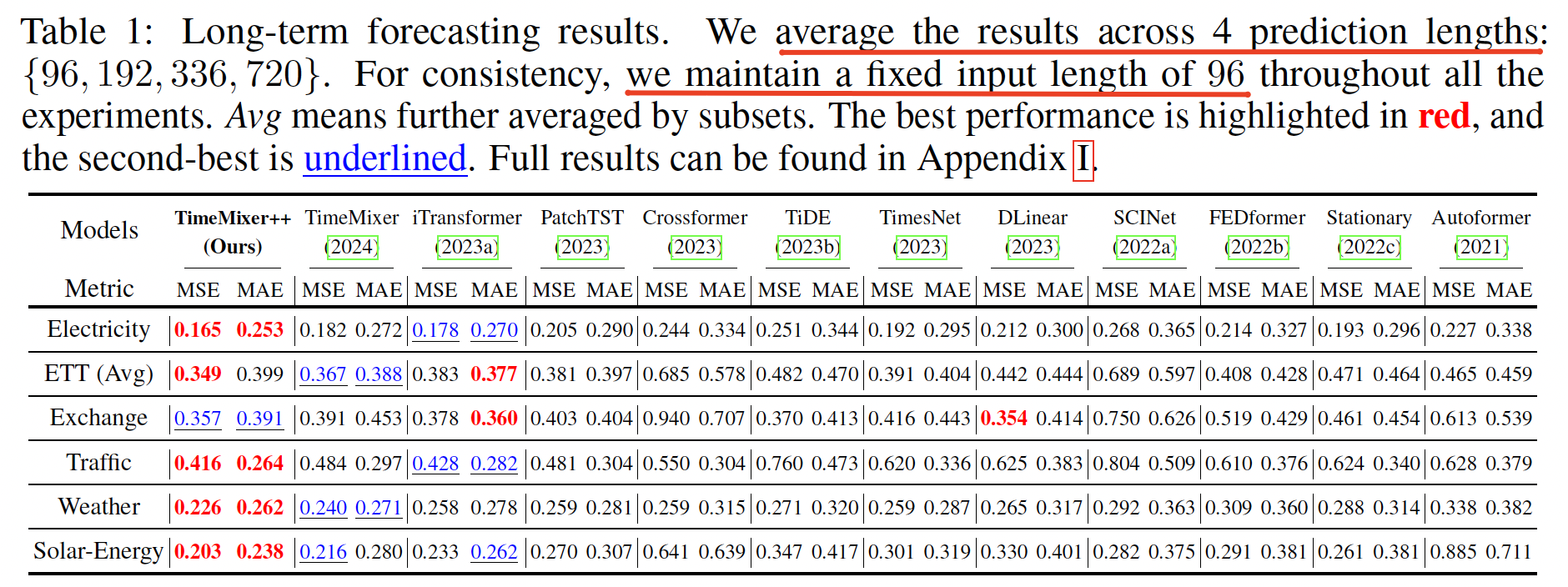
Task 2: Univariate short-term forecasting

Dataset: M4 Competition

Task 3: Multivariate short-term forecasting

Datset: PEMS03,04,07,08

Task 4: Imputation

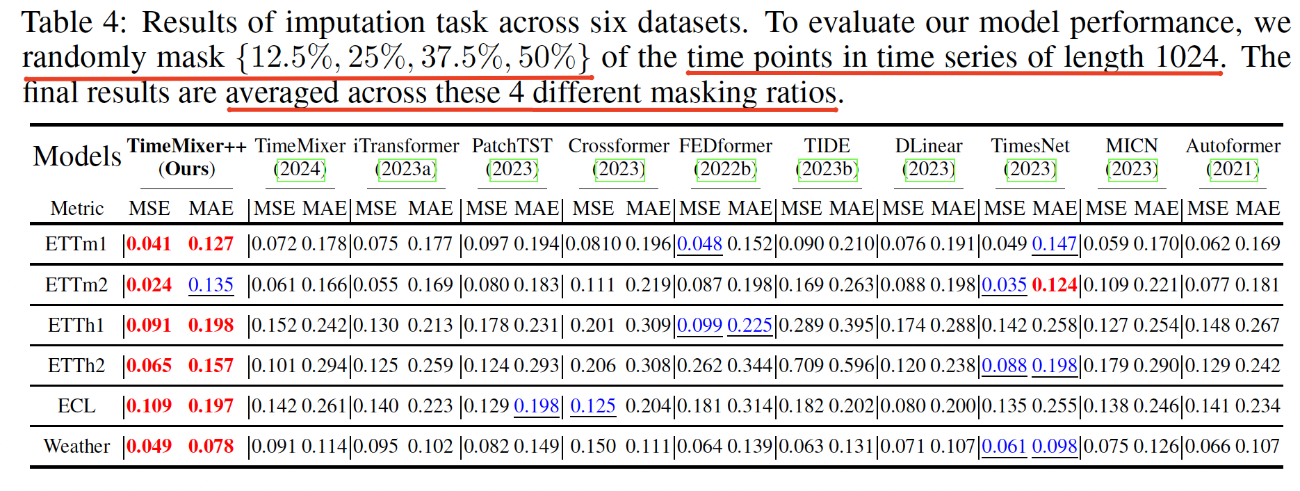
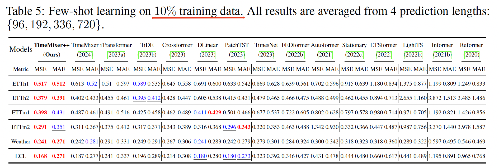
Task 5: Few-shot forecasting

Task 6: Zero-shot forecasting

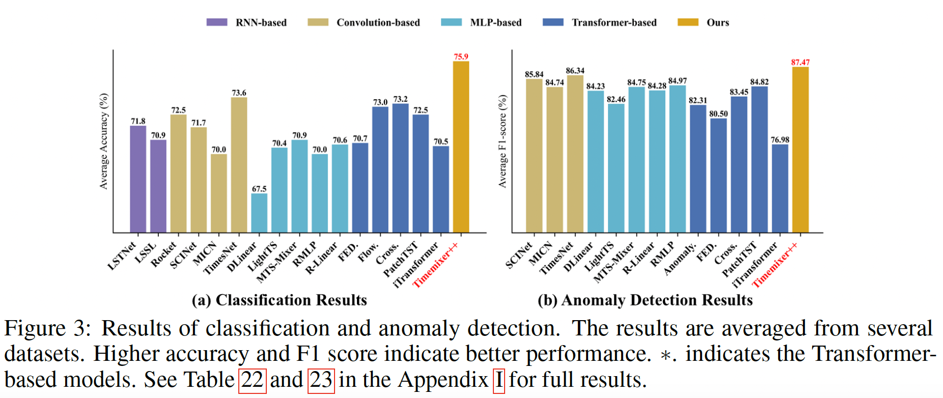
Task 7,8: Classifcation & Anomaly Detection

• Classification: 10 MTS datasets from UEA
• Anomaly detection: SMD (2019), SWaT (2016), PSM (2021), MSL and SMAP (2018).

(2) Model Analysis

a) Ablation Study

b) Representation Analysis

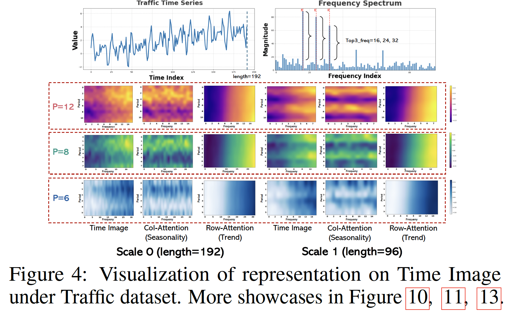
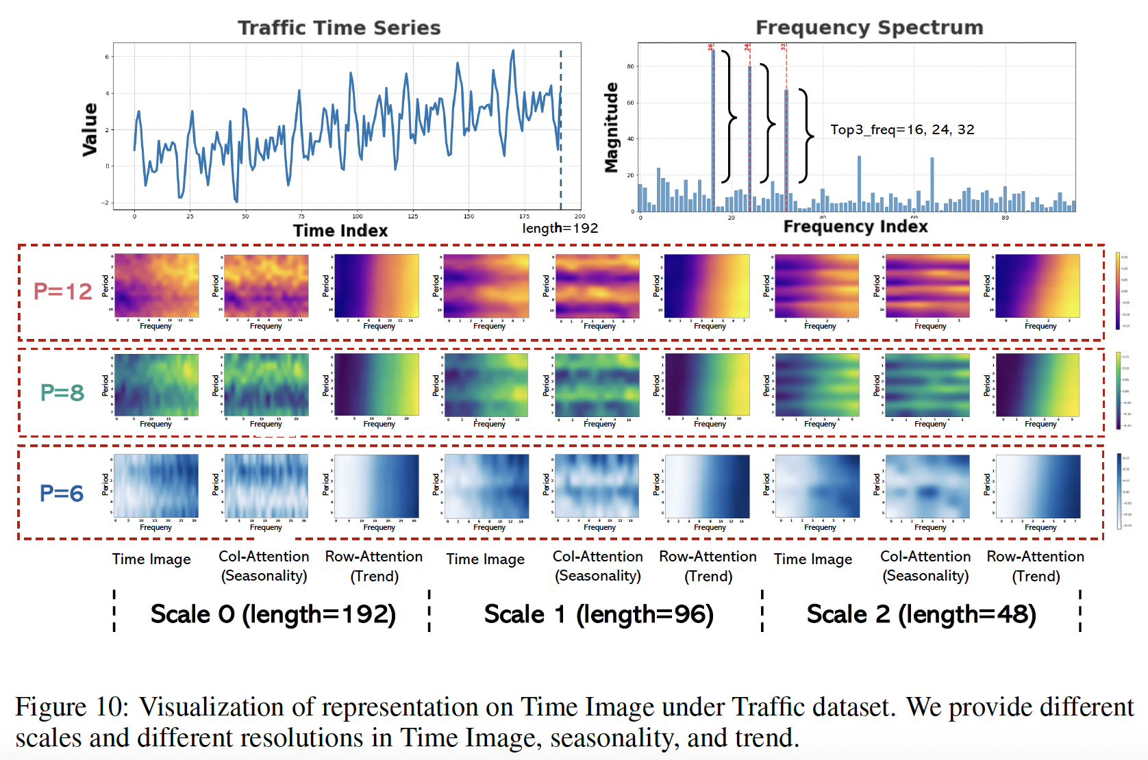
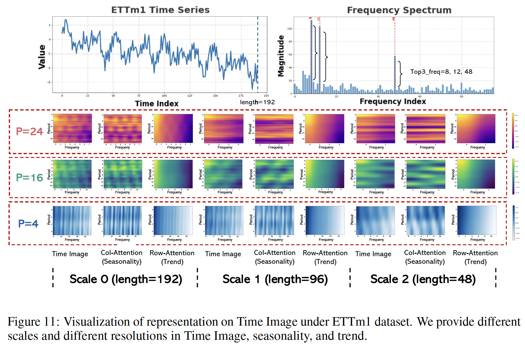
Presents the

• (1) Original image
• (2) Seasonality image
• (3) Trend image

across two scales and three resolutions

• (periods: 12, 8, 6; frequencies:16, 24, 32)

Result: Demonstrates efficacy in the separation of distinct seasonality and trends, precisely capturing multi-periodicities and time-varying trends.

• Periodic characteristics vary across different scales and resolutions.
• This hierarchical structure permits the simultaneous capture of these features, underscoring the robust representational capabilities of TimeMixer++ as a pattern machine

CKA between the representations from the first and last layers.

• (1) Superior performance in

  • prediction and anomaly detection with higher CKA similarity
  • imputation and classifcation with lower CKA similarity

• (2) Lower CKA similarity

  = More distinctive layer-wise representations

  = Suggesting a hierarchical structure

• (3) TimeMixer++

  • Captures distinct low-level representations for forecasting and anomaly detection
  • Captures hierarchical ones for imputation and classification

  \(\rightarrow\) Highlights TimeMixer++’s potential as a general TS pattern machine

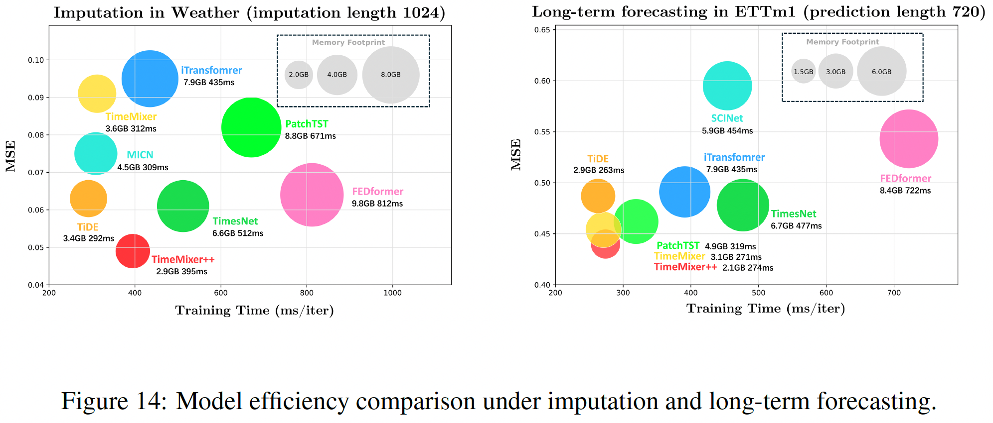
c) Efficiency Analysis

d) Additional Representation Anlayis