UniCL; A Universal Contrastive Learning Framework for Large Time Series Models

UniCL: A Universal Contrastive Learning Framework for Large Time Series Models

Contents

1. Abstract
2. Introduction
3. Foundation Models for TS Data
4. Framework Overview
5. Unified Foundation Model
6. Experiments

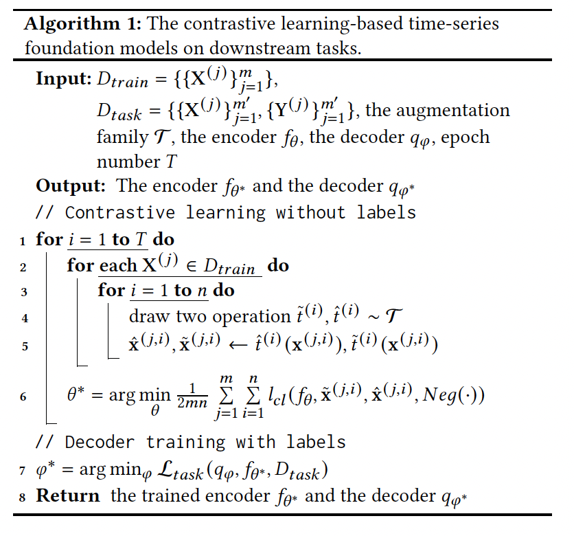
Abstract

Pre-trained Foundation Models (PFM)

• (1) leverages UNlabeled data
• (2) captures GENERAL TS patterns

Limitations of previous CL:

$\rightarrow$ Suffer from high-bias and low-generality issues, due to …

• (1) Use of predefined and rigid augmentation
• (2) Domain-specific data training

UniCL

• (1) Universal and scalable CL
• (2) PFM
• (3) Cross-domain datasets

Details

• (1) Unified and trainable “TS augmentation” operation

  • Generate pattern-preserved, diverse, and low-bias TS data
  • Leveraging spectral information

• (2) “Scalable augmentation” algorithm

  • Handle datasets with varying lengths

    ( facilitating cross-domain pretraining )

• Experiments) 2 benchmark datasets

  • across eleven domains

1. Introduction

Challenges in analyzing TS data:

• high dimensionality, noise, non-stationarity, periodicity, etc. [62].

TS analysis in DL

• (1) Supervised learning (SL)-based
• (2) PFM-based

Procedures of PFM:

• step 1) Pre-train on “TS data”
  • Capture the “general” intrinsic patterns of TS
• step 2) Fine-tune on “specific TS tasks”

Mask-based pre-training approaches: Limitations?

• Require numerous unlabeled TS data
• TS are scarce in the open-world website

\(\rightarrow\) Achieve suboptimal performance!

To alleviate the heavy reliance on numerous TS data…

\(\rightarrow\) CL approaches are proposed to “augment TS”

• step 1) Generate views
• step 2) CL loss

Limitations of CL-based PFMs

• (1) High-bias & Low-generality

  • TS augmentation operations

    ( ex. permutation [41, 47], random masking [63, 72], and warping [14] )

    • ignore the TS intrinsic properties (ex. periodicity)

      \(\rightarrow\) Introduce high bias and noise

    • ex) permutation shuffles the sequential information

• (2) Generally pretrained within a single domain

  • TS can vary significantly across different domains!

    \(\rightarrow\) Fail to transfer!

(1) UniCL

Universal PFM for TS analysis

(Solution 1) High-bias

• Use effective “pattern-preserved augmentation” operations

  \(\rightarrow\) Capable of learning the intrinsic patterns

(Solution 2) Low-generality

• Use data of “various domains”

  \(\rightarrow\) Generalize on various domains

Three technical challenges

• [A] No theoretical analysis and established metrics for “preserving the patterns of TS data” with DL
  • Cannot design effective augmentation operations
• [B] “High variations” in TS data from different domains (i.e. different length)
  • Challenging to design a scalable and unified augmentation algorithm
• [C] Existing studies) Train the LLM-based encoder by optimizing the “predictive objective”
  • Less attention in contrastive objective

Three Solutions

• [A] Empirically reveal a “positive” correlation between

  • a) Bias of TS embeddings
  • b) Spectral distance between augmented and raw TS

  \(\rightarrow\) Propose a unified and trainable TS augmentation operation & two novel losses

• [B] “Scalable and unified augmentation”

  • utilizes spectrum preserved TS segmentation

• [C] “Transformer”-based encoder

  • 40 cross-domain datasets
  • Initialized with pre-trained weights from the text encoder of CLIP

(2) Contributions

(1) General framework for PFM based on CL

• capable of handling high variation TS

(2) Reveal the factor of representation bias based on a novel metric

• ( + propose a unified and trainable augmentation )
• ( + propose two novel losses )

(3) Handle data with “varied length”

• by pattern-preserved segmentation and concatenation
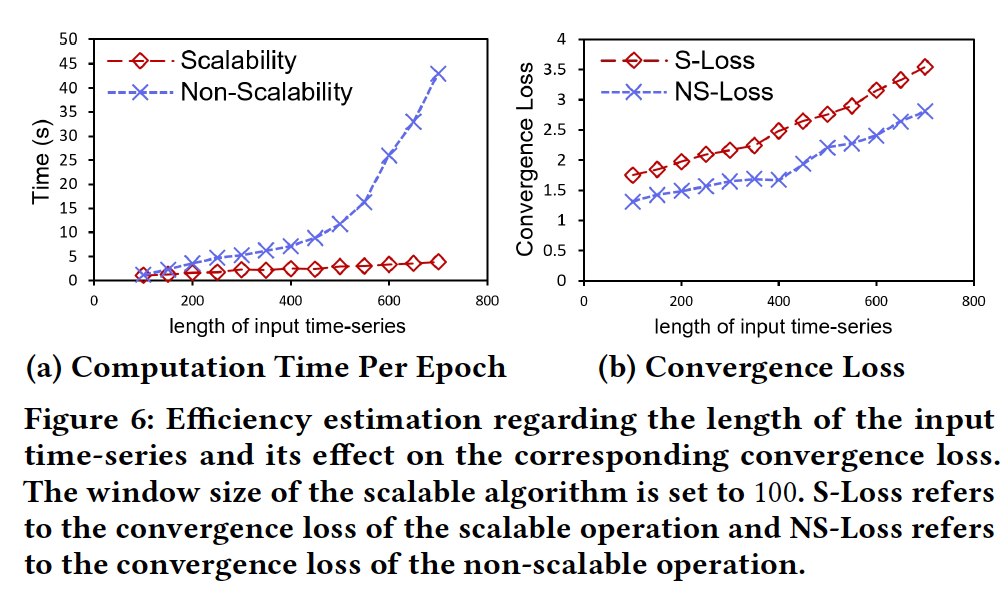
• demonstrate bounded convergence loss differences between scalable and non-scalable algorithms

(4) First to train the LLM backbone with “CL loss” for general TS

• 40 cross-domain datasets
• 2 downstream tasks

2. Foundation Models for TS Data

(1) PFMs

Three types

• (1) LLM-based
• (2) Mask-based
• (3) CL-based

a) LLM-based

Naive approach

• step 1) Take pretrained LLMs as the foundation model \(f_{\theta^*}\)
• step 2) Propose to apply it on the TS

ex) LLMTIME [42]

• Encodes TS as a “string” of numerical digits

  ( with each digit separated by spaces )

ex) LSTPrompt [32], PromptCast [70]

• Incorporate domain information and frequency into “template-based” descriptions
• Embed them using a “text tokenizer” to guide the LLM

Limitation)

• Inherently designed for handling text data

  ( = discrete and categorical )

Solution)

• Mask-based [12,74]
• CL based [72,78]

b) Mask-based

Classified into

• (1) Reconstruction based [12,16,28,74]
• (2) **Prediction **based [3,22,37]

Procedures

• step 1) Random mask \(\mathrm{M} \in\{0,1\}^{n \times T}\)
  • Masking: \(\mathrm{X}^{(j)} \odot \mathrm{M}^{(j)}\).
• step 2)
  • (1) Reconstruction loss
    • \(\mathcal{L}_{r l}=\frac{1}{m} \sum_{j=1}^m\left\|\mathrm{X}^{(j)} \odot\left(1-\mathrm{M}^{(j)}\right)-\hat{\mathrm{X}}^{(j)} \odot\left(1-\mathrm{M}^{(j)}\right)\right\|_2^2\).
  • (2) Prediction loss
    • \(\mathcal{L}_{p l}=\frac{1}{m} \sum_{j=1}^m\left\|\mathrm{X}_{t: t+H_f}^{(j)}-\hat{\mathrm{X}}_{t: t+H_f}^{(j)}\right\|_2^2\).

Limitation)

• (1) Necessitates abundant data
  • Due to its reliance on self-encoding reconstruction and prediction objectives
• (2) Masked values are often easily predicted from neighbors

Solution)

• Large-scale datasets

c) CL-based

Mainly differ in “positive view generation”

Classified into 2 types

• (1) Context-based [25, 60, 72]
• (2) Augmentation-based

(1) Context-based

• generally advocate contextual consistency

  ( sub-series with close temporal relationships = positive views )

• ex) TS2Vec [72]
  • two overlapping time segments
• ex) others [25, 60]
  • opt for temporal neighborhood sub-series
• Limitation)
  • Rely on observed data
  • Perform poorly on unseen data

(2) Augmentation-based

• Generate diverse TS based on observed data
• ex) Predefined data augmentation operation
  • jittering [13, 52, 71], scaling [66], permutation [41, 47], magnitude warping [14], masking [63, 72], and pooling [29]

• ex) Perturbation in the frequency domain [33, 78]

• ex) CLUDA [46]
  • adopts a composition of operations to generate positive views.
• Limitation)
  • Dependence on expert knowledge [40]
  • Susceptible to inductive bias [56]
• ex) meta-learning [39] to select augmentation operations adaptively based on criteria of fidelity and variety.

\(\rightarrow\) Still rely on a pre-defined set of augmentations

(2) Fine-tuning TS Foundation Model

• Partial Fine-tunining (P-FT)
• Full Fine-Tuning (F-FT) \(\rightarrow\) This paper

(3) Variable Independence

Transformer-based learning :

variable-mixing (or channel-mixing)

• \(\mathrm{X} \in \mathbb{R}^{n \times T}\) is mapped into \(\mathbf{Z} \in \mathbb{R}^{T \times D}\)

• Two critical issues:

  • (1) The embedding layer requires the pre-definition of the number of variables

    \(\rightarrow\) lacks generality for cross-domain

  • (2) A timestamp-wise shared embedding space may not be suitable for all domains

    • as the mechanism of dependency can vary

      (e.g., lag-features of financial time-series [53])

UniCL: “variable independence” configuration

( = processing \(n\) variables independently )

3. Framework Overview

UniCL

• (1) Universal CL framework designed for TS analysis
• (2) Handle heterogeneous cross-domain TS
• (3) Unified augmentation operation

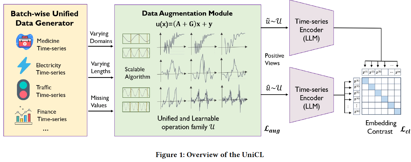
Four steps:

• (1) Data generation
• (2) Data augmentation
• (3) TS encoder based on LLMs
• (4) Contrastive learning

Procedures

• Step 1) TS from diverse domains
  • Partitioned into batches
• Step 2) Augmentation module
  • Varying lengths of inputs with missing values
  • Unified and learnable augmentation operation
• Step 3) CLIP-based encoder
  • generates embeddings for all views
• Step 4) CL loss

4. Unified Foundation Model

4.1) Observations about the “bias” in TS representation

• caused by “pre-determined” augmentation methods

4.2) Summarize existing methods & propose a unified and learnable augmentation operation family

• Introduce two novel efficient loss functions
• Scalable version of this unified operation set
  • to handle datasets from various domains with different lengths and missing values.

4.3) Introduce the encoder of the UniCL & whole pre-training paradigm

(1) A Unified Data Augmentation Operation

Existing pre-defined TS augmentation methods

\(\rightarrow\) introduce an “inductive bias”

(Key motivational observation)

Bias in TS embedding correlates “positively” with the spectral distance (SD) between raw and augmented series

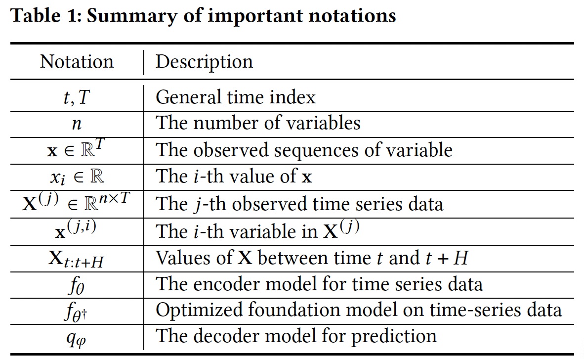
Notation

• \(\mathcal{T}(\cdot)\): pre-defined data augmentation family

• \(\left\{t^{(k)}\left(\mathbf{x}^{(j, i)}\right)\right\}_{k=1}^K\): augmentation set of \(\mathbf{x}^{(j, i)}\)
  • with size \(K\), where \(t^{(k)} \sim \mathcal{T}\).

• \(\mathcal{T}\left(\mathbf{x}^{(j, i)}\right)\): transformation distribution of \(\mathbf{x}^{(j, i)}\).

• \(\mathcal{F}(\cdot)\): FFT

• $$

  \cdot

  $$ : amplitude operator

  • $$

    \cdot

    =\(\)\sqrt{\mathcal{R}(\cdot)^2+\mathcal{J}(\cdot)^2}$$,

    • \(\mathcal{R}(\cdot)\) and \(\mathcal{J}(\cdot)\) : real and imaginary part operators

  • $$

    \cdot

    $$ operator: only generates the first half and removes the zero-frequency component

    ( i.e., $$

    \cdot

    : \mathbb{C}^T \rightarrow \mathbb{R}^{\left\lfloor\frac{T}{2}\right\rfloor}$$ )

[1] Bias introduced by \(\mathcal{T}(\cdot)\)

• \(\begin{aligned} \operatorname{Bias}\left(\mathcal{T}\left(\mathbf{x}^{(j, i)}\right)\right) & =\left\|\mathbb{E}_{\boldsymbol{t} \sim \mathcal{T}}\left[f_\theta\left(t\left(\mathbf{x}^{(j, i)}\right)\right)\right]-f_\theta\left(\mathbf{x}^{(j, i)}\right)\right\|_2 \\ & \approx\left\|\frac{1}{K} \sum_{k=1}^K f_\theta\left(t^{(k)}\left(\mathbf{x}^{(j, i)}\right)\right)-f_\theta\left(\mathbf{x}^{(j, i)}\right)\right\|_2 \end{aligned}\).

[2] Spectral distance between \(\mathbf{x}^{(j, i)}\) and \(t\left(\mathbf{x}^{(j, i)}\right)\)

• $$S D\left(\mathbf{x}^{(j, i)}, t\left(\mathrm{x}^{(j, i)}\right)\right)=\left|\left

  \mathcal{F}\left(\mathrm{x}^{(j, i)}\right)\right

  -\left

  \mathcal{F}\left(t\left(\mathrm{x}^{(j, i)}\right)\right)\right

  \right|_2^2$$.

Settings

• Model: TS2Vec
• 4 pre-defined augmentation methods
  • jittering, scaling, time warping, and permutation
• 23 selected MTS from UEA
• Report the average bias and spectral distance
• Output layer of the encoder = 2D for viz
• Generate \(K=500\) augmented samples randomly for each sample, and compute the ..
  • (1) Average bias: \(\frac{1}{m n} \sum_{j=1}^m \sum_{i=1}^n \operatorname{Bias}\left(\mathcal{T}\left(\mathbf{x}^{(j, i)}\right)\right)\)
  • (2) Average spectral distance: \(\frac{1}{m n K} \sum_{j=1}^m \sum_{i=1}^n \sum_{k=1}^K S D\left(\mathbf{x}^{(j, i)}, t^{(k)}\left(\mathbf{x}^{(j, i)}\right)\right)\)

Result:

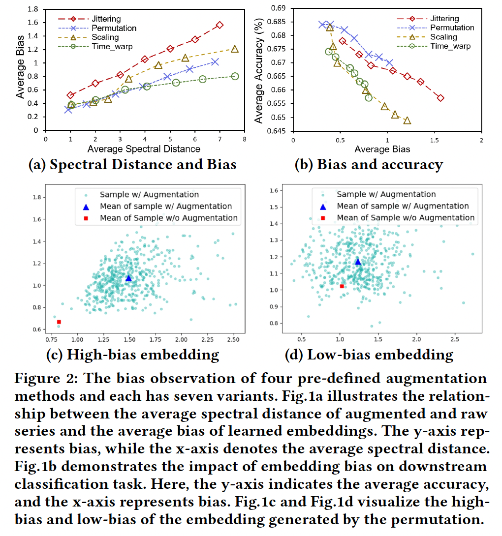
• (a) positive correlation

• (b) Higher bias \(\rightarrow\) Reduced performance

  ( on downstream classification tasks )

  \(\rightarrow\) motivate the need for TS augmentation methods to control the spectral distance between augmented and raw time-series.

• (c,d) significant bias may hinder the effectiveness of separating augmented embeddings across different instances

  \(\rightarrow\) limiting the discriminative power of learned embeddings

Unified DA operation

[1] Naive approach) Employ all augmentation operations

[2] Limitation) Hyper-parameter space can be continuous

(e.g., standard deviation of jittering, number of speed changes of time warping)

\(\rightarrow\) making it infeasible to explore the full augmented view space

[3] Solution

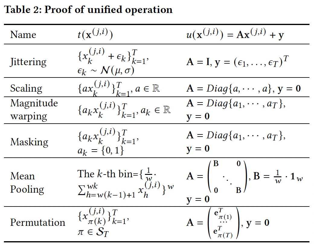
• Introduce a unified operation family \(\mathcal{U}\).

• Given input \(\mathbf{x}^{(j, i)}\) & \(u \sim \mathcal{U}\) ,

  \(u\left(\mathbf{x}^{(j, i)}\right)=\mathbf{A} \mathbf{x}^{(j, i)}+\mathbf{y}\).

  • where \(\mathbf{x}^{(j, i)} \in \mathbb{R}^T, \mathbf{A} \in \mathbb{R}^{T \times T}\) and \(\mathbf{y} \in \mathbb{R}^T\).

• [Proposition 1] Operation \(u \sim \mathcal{U}\) yield an augmented view space equivalent to that of each pre-defined operation and their compositions.

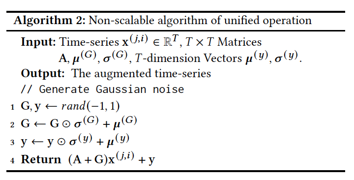
To introduce randomness ….

• incorporate a “random” matrix \(\mathrm{G}\) with the “deterministic” matrix A.

Non-scalable unified operation

• (vector) \(u\left(\mathbf{x}^{(j, i)}\right)=(\mathbf{A}+\mathbf{G}) \mathbf{x}^{(j, i)}+\mathbf{y}\).
• (matrix) \(u\left(\mathrm{X}^{(j)}\right)=\mathrm{X}^{(j)}(\mathrm{A}+\mathrm{G})^T+\mathrm{y}\).

• time and space complexity: \(O\left(4 T^2+3 T\right)\)

  \(\rightarrow\) Scalable and efficient algorithms in Section 4.2

• [Proposition 2] The transformation distribution \(\mathcal{U}\left(\mathrm{x}^{(j, i)}\right)\) follows MVN

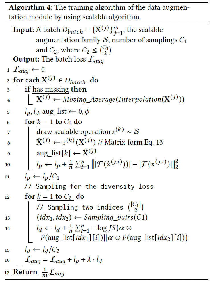
(2) Scalable and Diverse DA

(1) Propose DA objective based on our proposed unified operation

• to generate (1) spectrum-preserved and (2) diverse TS

(2) Propose a scalable algorithm to apply this objective to TS with various lengths

a) Spectrum-preserved and Diverse Objective

Two properties of DA

• (1) Pattern preservation
• (2) Diversity

Two novel losses

• (1) Spectrum-preservation loss \(l_p\)
• (2) Spectrum-diversity loss

(1) Spectrum-preservation loss \(l_p\)

• To generate “low-bias” embeddings, p

  positive pairs should be close to the original series “in terms of spectral distance”

• \(\begin{aligned} l_p\left(\mathcal{U}, \mathbf{x}^{(j, i)}\right)= & \frac{1}{2} \mathbb{E}_{\tilde{\mathcal{U}} \sim} \mathcal{U}\left[\left\|\left|\mathcal{F}\left(\tilde{u}\left(\mathbf{x}^{(j, i)}\right)\right)\right|-\left|\mathcal{F}\left(\mathbf{x}^{(j, i)}\right)\right|\right\|_2^2\right] \\ & \quad+\frac{1}{2} \mathbb{E}_{\hat{u} \sim \mathcal{U}}\left[\left\|\left|\mathcal{F}\left(\hat{u}\left(\mathbf{x}^{(j, i)}\right)\right)\right|-\left|\mathcal{F}\left(\mathbf{x}^{(j, i)}\right)\right|\right\|_2^2\right] \\ = & \mathbb{E}_{\mathcal{u} \sim} \mathcal{U}\left[\left\|\left|\mathcal{F}\left(u\left(\mathbf{x}^{(j, i)}\right)\right)\right|-\mid \mathcal{F}\left(\mathbf{x}^{(j, i)}\right)\right\|_2^2\right] \end{aligned}\).

(2) Spectrum-diversity loss

• a) Metric to quantify the diversity
• b) Identify which patterns in \(\mathbf{x}^{(j, i)}\) are not essential

Candidates

• a-1) Average entropy

  • \(\frac{1}{T} \sum_{k=1}^T \ln \left(2 \pi e \sigma_k^2\right)\), where \(\sigma_k^2=\sum_{h=1}^T\left(\sigma^{(G)}[k][h]\right)^2\) \(x_h^{(j, i)}+\left(\sigma_k^{(y)}\right)^2\).
  • HOWEVER … simply increasing the entropy of each point results in large \(\sigma^{(G)}\) and \(\sigma^{(y)}\), introducing meaningless noise

• a-2) Average KL-divergence

  • \(\frac{1}{T} \sum_{k=1}^T K L(P(\tilde{x}_k^{(j, i)} \| P\left(\hat{x}_k^{(j, i)}\right))\).
  • HOWEVER infeasible!! … in TS, only one observation is available at each timestamp

• a-3) Solution: transform the positive views \(\tilde{\mathbf{x}}^{(j, i)}\) and \(\hat{\mathbf{x}}^{(j, i)}\) into the frequency domain

  • $$\left

    \mathcal{F}\left(\tilde{\mathbf{x}}^{(j, i)}\right)\right

    \(and\)\left

    \mathcal{F}\left(\hat{\mathbf{x}}^{(j, i)}\right)\right

    $$,

  • \(k\)-th element $$\left

    \mathcal{F}\left(\tilde{\mathbf{x}}^{(j, i)}\right)\right

    _k\(and\)\left

    \mathcal{F}\left(\hat{\mathbf{x}}^{(j, i)}\right)\right

    _k$$

    • denoting the amplitude of the \(k\)-th frequency component
  • convert the amplitude sequence to a probability mass function (PMF)

    • $$P\left(\tilde{\mathbf{x}}^{(j, i)}\right)=\operatorname{Softmax}\left(\left

      \mathcal{F}\left(\tilde{\mathbf{x}}^{(j, i)}\right)\right

      / \tau\right)$$.

    • $$P\left(\hat{\mathbf{x}}^{(j, i)}\right)=\operatorname{Softmax}\left(\left

      \mathcal{F}\left(\hat{\mathbf{x}}^{(j, i)}\right)\right

      / \tau\right)$$.

  • measure the diversity by calculating JS-divergence

  • but not all the frequency component should be diversified!

    \(\rightarrow\) multiply the PMF by a decay factor \(\boldsymbol{\alpha}=\left[\alpha_1, \alpha_2, \cdots, \alpha_{\left\lfloor\frac{T}{2}\right]}\right]^T\)

• Result: \(\begin{aligned} & l_d\left(\mathcal{U}, \mathbf{x}^{(j, i)}, \boldsymbol{\alpha}\right)= \\ & \mathbb{E}_{(\tilde{u}, \hat{u}) \sim \mathcal{U}}\left[-\log J S\left(\boldsymbol{\alpha} \odot P\left(\tilde{u}\left(\mathbf{x}^{(j, i)}\right)\right) \| \boldsymbol{\alpha} \odot P\left(\hat{u}\left(\mathbf{x}^{(j, i)}\right)\right)\right)\right] \end{aligned}\)

  • where $$P(\cdot)=\operatorname{Softmax}(

    \mathcal{F}(\cdot)

    / \tau)$$

  • \(\log\) is used to stabilize the optimization.

[Summary]

\(\mathcal{L}_{\text {aug }}\left(\mathcal{U},\left\{\mathbf{X}^{(j)}\right\}_{j=1}^m, \boldsymbol{\alpha}\right)=\sum_{j=1}^m \sum_{i=1}^n l_p\left(\mathcal{U}, \mathbf{x}^{(j, i)}\right)+\lambda \cdot l_d\left(\mathcal{U}, \mathbf{x}^{(j, i)}, \boldsymbol{\alpha}\right)\).

b) Scalable operations

Q) How we can efficiently employ it in TS datasets with high variations? (i.e. Varying sequence lengths)

Two key issues need to be addressed:

• (1) Lengthy TS \(\mathbf{x}^{(j, i)} \in \mathbb{R}^T\)
• (2) Employing different size of unified operation for each dataset is inefficient.

\(\rightarrow\) Introduce a scalable algorithm that offers efficient implementation

• requires only a fixed-size unified operation
• results) space complexity of \(O\left(K^2\right)\), where \(K\) is a constant.

Fix-sized unified operation:

• \(u\left(\mathbf{x}^{(j, i)}, k\right)=\left(\mathrm{A}_{k \times k}+\mathrm{G}_{k \times k}\right) \mathbf{x}_{k \times 1}^{(j, i)}+\mathbf{y}_{k \times 1}\).
• Can only handle input TS with a fix length \(K\) …. Solution?

(When \(T<K\)) employ iterative extension via repetition

• aligns with the periodicity assumption of Fourier analysis, ensuring \(x_i=x_{i+T}\),

• padding: may disrupt the spectrum pattern of \(\mathbf{x}\) )

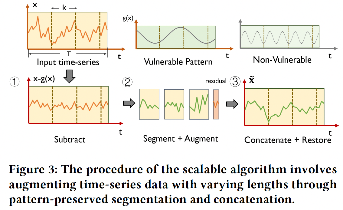
(When \(T>K\)) segmentation to the input TS … Figure 3

• Step 1) \(g(\mathrm{x})\) : vulnerable pattern which will be disrupted by segmentation. Thus, should be …
  • a) subtracted prior to the segmentation
  • b) restored after concatenation
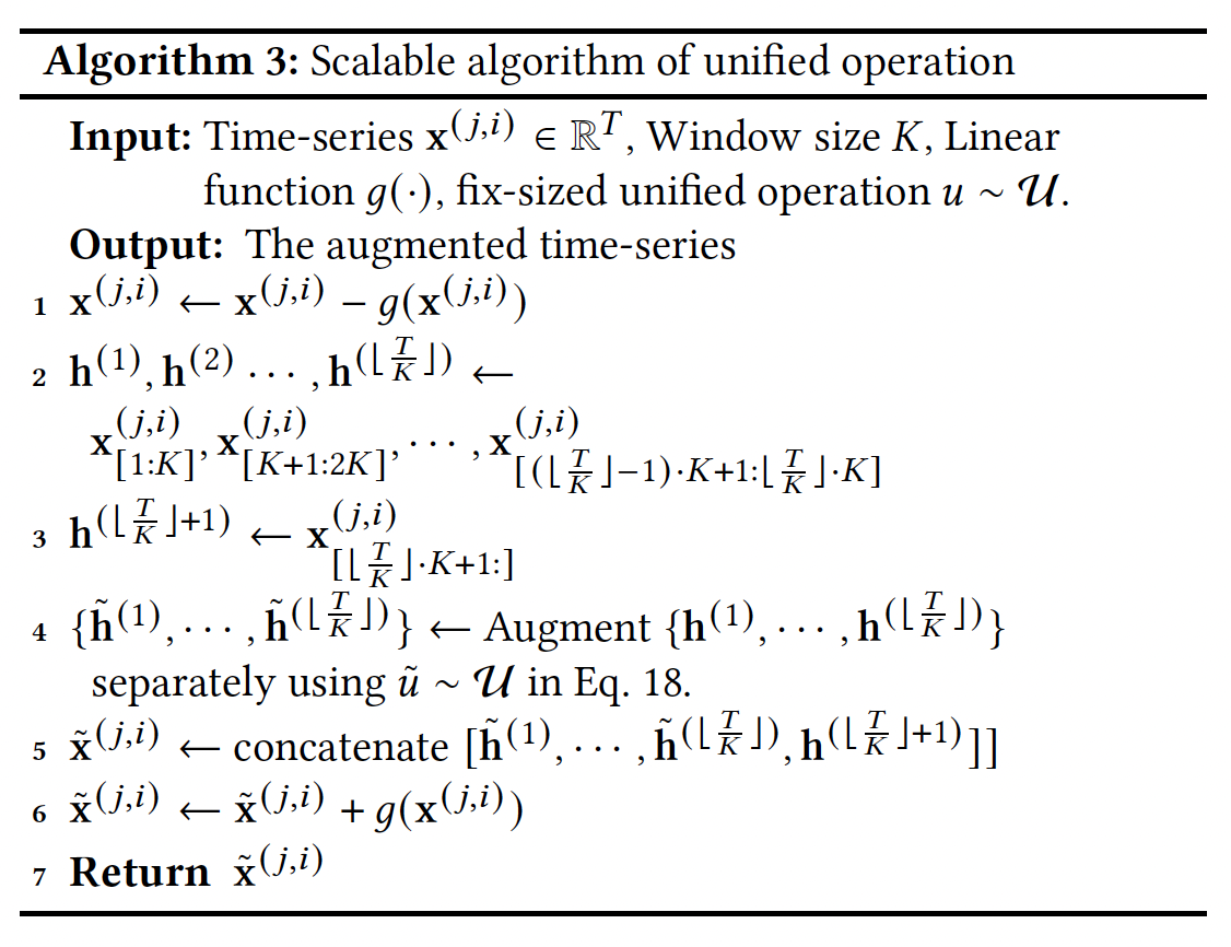
• Step 2) segment the TS into \(\left\lfloor\frac{T}{K}\right\rfloor+1\) non-overlapping subseries
  • \(\left\{\mathbf{h}^{(l)} \in \mathbb{R}^K, \left.\mathbf{h}^{\left(\left\lfloor\frac{T}{K}\right\rfloor+1\right)} \right\rvert\, l=1, \cdots,\left\lfloor\frac{T}{K}\right\rfloor\right\}\) .
  • where \(\mathbf{h}^{\left(\left\lfloor\frac{T}{K}\right\rfloor+1\right)} \in\) \(\mathbb{R}^{r e s}\) is the residual term and \(0 \leq r e s<K\).
• Step 3) Augment each subseries separately
  • using fix-sized unified operation
• Step 4) Concatenate them in the same order
  • \(\tilde{\mathbf{x}}^{(j, i)}=\) \(\left[\tilde{u}^{(1)}\left(\mathbf{h}^{(1)}, k\right), \cdots, \tilde{u}^{\left(\left\lfloor\frac{T}{K}\right\rfloor\right)}\left(\tilde{\mathbf{h}}^{\left(\left\lfloor\frac{T}{K}\right\rfloor\right)}, k\right), \mathbf{h}^{\left(\left\lfloor\frac{T}{K}\right\rfloor+1\right)}\right]\), where \(\tilde{u} \sim \mathcal{U}\).

Segmenting the time-series into \(K\) non-overlapping subseries

\(\rightarrow\) may disrupt the \(\left\lfloor\frac{T}{K}\right\rfloor\) lowest frequency components

\(\rightarrow\) Solution) define the linear function \(g(\cdot)\) to extract the lowest \(\left\lfloor\frac{T}{K}\right\rfloor\) frequency components, thereby preserve such vulnerable patterns.

The \(k\)-th value of function \(g(\cdot)\) :

• \(g\left(\mathbf{x}^{(j, i)}\right)[k]=\sum_{h=0}^{\left\lfloor\frac{T}{K}\right\rfloor} 2 \cdot a m p_h \cdot \cos \left(2 \pi f_h(k-1)+\phi_h\right)\).

Missing values.

• may contain missing values requiring imputation
• motivation)
  • low-frequency components: carry essential information
  • high-frequency components: often introduce noise.
• result)
  • step 1) Linear interpolation
  • step 2) Apply a moving average with a window size of 10.

(3) Pre-train LLM

a) Encoder

Encoder function \(f_\theta: \mathbb{R}^{n \times T} \rightarrow \mathbb{R}^{n \times P \times D}\).

• (1) Input embedding layer
  • Partition the input positive views generated by the augmentation module
    • positive views \(\tilde{\mathrm{X}}^{(j)}\) and \(\hat{\mathrm{X}}^{(j)}\)
      • length of \(L_p\)
      • # of patches \(P\)
  • Transform the \(\tilde{\mathrm{X}}_p^{(j)}, \hat{\mathrm{X}}_p^{(j)} \in \mathbb{R}^{n \times P \times L_p}\) into the high-dimensional space \(\tilde{\mathbf{H}}_p^{(j)}, \hat{\mathbf{H}}_p^{(j)} \in \mathbb{R}^{n \times P \times D}\).
• (2) Causal transformer encoder blocks
  • both \(\tilde{\mathbf{H}}_p^{(j)}\) and \(\hat{\mathbf{H}}_p^{(j)}\) are fed
  • architecture of the text encoder in ViT-G/14 CLIP
    • 32 transformer blocks with 1280 hidden dimensions
  • opt for ViTG/14’s text encoder structure due to our shared contrastive-based pre-training paradigm and mutual need for sequence modeling.
  • output) patch-wise embeddings \(\tilde{\mathbf{Z}}^{(j)}, \hat{\mathbf{Z}}^{(j)} \in \mathbb{R}^{n \times P \times D}\). I

b) Contrastive Loss

Hierarchical contrastive loss \(\mathcal{L}_{c l}\)

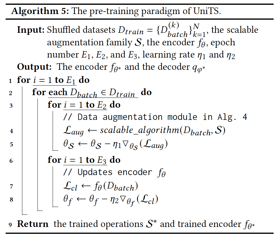
c) Pre-training paradigm

Wide range of TS data

• \(D_{\text {train }}=\left\{D_1, D_2, \cdots, D_N\right\}\).

Preprocess all the TS data into batches

• \(D_i \rightarrow\left\{\right.\) batch \(_1^{(i)}\), batch \(\left._2^{(i)}, \cdots\right\}\),
  • where each batch from different domains contain varying length

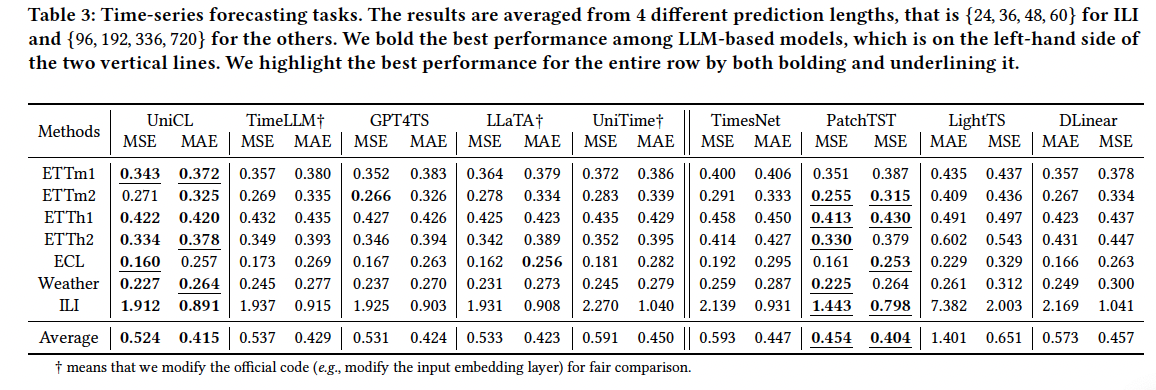
5. Experiments

• TS forecasting
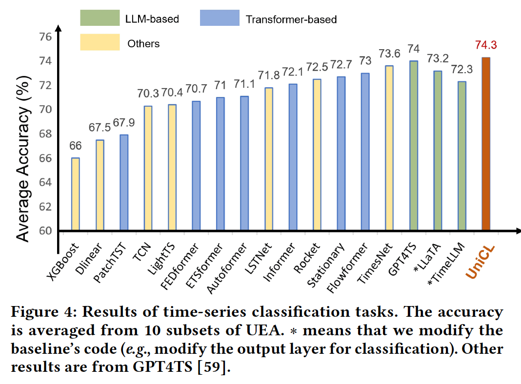
• TS classification
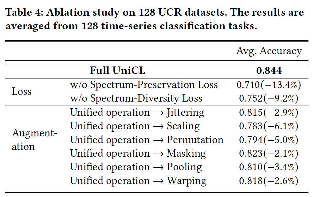
• Ablation analyses
  • to assess the scalability and efficacy of the proposed data augmentation methods.

Implementation details

• pre-training on 40 cross-domain datasets sourced from the Monash Time Series Forecasting Repository
  • varying lengths, ranging from 2 to 7𝑀,
  • include missing values, with missing rate ranging from 2% to 17%.
• pre-train the model on four NVIDIA A800 GPU for one week

• time cost per epoch