Unified Training of Universal Time Series Forecasting Transformers

Unified Training of Universal Time Series Forecasting Transformers

Contents

1. Abstract
2. Introduction
3. Reatled Work
4. Method
   1. Problem Formulation
   2. Architecture
   3. Unified Training
5. Experiments
   1. In-distribution Forecasting
   2. OOD / Zero-shot Forecasting
   3. Ablation Study

Abstract

Universal forecasting,

• Pre-training on a vast collection of TS datasets
• Large Time Series Model

Challenges

• (1) Cross-frequency learning
• (2) Arbitrary number of variates for MTS
• (3) Varying distributional properties inherent in large-scale data.

Masked EncOder-based UnIveRsAl TS Forecasting Transformer (MOIRAI)

Dataset: Large-scale Open Time Series Archive (LOTSA)

• featuring over 27B observations
• across 9 domains

1. Introduction

Universal forecasting paradigm

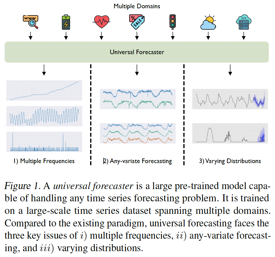
Challenges: highly heterogeneous.

(1) Frequency

\(\rightarrow\) Cross-frequency learning has been shown to be a challenging!

• Due to negative interference (Van Ness et al., 2023)
• Existing work) simply avoiding this problem
  • just learn one model per frequency

(2) Dimensionality

• While considering each variate of a multivariate time series independently can sidestep this problem, we expect a universal model to be sufficiently flexible to consider multivariate interactions & exogenous covariates

(3) Probabilistic forecasting

(4) Requires a large-scale dataset from diverse domains

Masked Encoder

Novel modifications

( to handle the heterogeneity of arbitrary TS data )

• (1) “Multiple” input and output projection layers
  • To handle varying frequencies
  • use patch-based projections with larger patch sizes for high-frequency data
• (2) Any-variate Attention,
  • To address the problem of varying dimensionality
  • simultaneously considers both time and variate axes as a single sequence
    • Rotary Position Embeddings (RoPE) (Su et al., 2024) \(\rightarrow\) to encode TIME axes
    • learned binary attention biases (Yang et al., 2022b) \(\rightarrow\) to encode VARIATE axes
• (3) Mixture of parametric distributions
  • To overcome the issue of requiring flexible predictive distributions
• (4) Others: optimizing the NLL of a flexible distribution

2. Related Work

(1) Pre-training for Zero-shot Forecasting

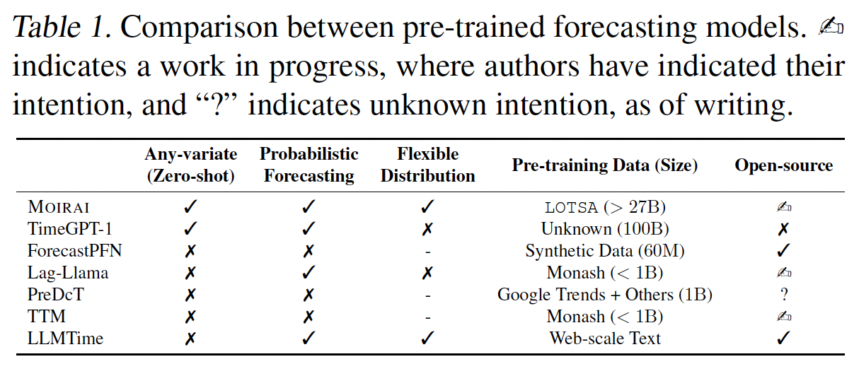
TimeGPT-1 (Garza & Mergenthaler-Canseco, 2023)

• first presented a closed source model

• zero-shot forecasting

  ( + fine-tuning through an API )

ForecastPFN (Dooleyet al., 2023)

• pre-train on synthetic TS
  • which can be subsequently be leveraged as a zero-shot forecaster
  • specialized for data or time limited settings

Lag-llama (Rasul et al., 2023)

• foundation model for TS forecasting
• leveraging the LLaMA (Touvron et al., 2023) architecture
• use lagged TS features
• presents neural scaling laws for TS forecasting

PreDcT (Das et al., 2023b)

• patch-based decoder-only foundation model for TS forecasting
• larger output patch size for faster decoding
• Dataset) private dataset from Google Trends + opendata

Tiny Time Mixers (TTMs) (Ekambaram et al., 2024)

• concurrent work leveraging lightweight mixer-style architecture.
• data augmentation by downsampling high-frequency TS
• support multivariate downstream tasks
  • by fine-tuning an exogenous mixer

LLMTime (Gruver et al., 2023)

• treats TS as strings
• apply careful pre-processing based on the specific LLMs’ tokenizer

(2) Pre-train + Fine-tune for TS Forecasting

Denoising autoencoders (Zerveas et al., 2021)

Contrastive learning (Yue et al., 2022; Woo et al., 2021)

\(\rightarrow\) Pre-training and fine-tuning on the same dataset

SimMTM

• combining both reconstruction and contrastive based pre-training approaches
• initial explorations into cross-dataset transfer

Reprogramming

• fine-tuning the model weights of an LLM for downstream tasks for other modalities
• ex) Zhou et al. (2023), Jin et al. (2023)
  • introduce modules and fine-tuning methods to adapt LLMs for TS tasks

3. Method

(1) Problem Formulation

Dataset of \(N\) time series \(\mathcal{D}=\left\{\left(\boldsymbol{Y}^{(i)}, \boldsymbol{Z}^{(i)}\right)\right\}_{i=1}^N\),

• \(\boldsymbol{Y}^{(i)}=\) \(\left(\boldsymbol{y}_1^{(i)}, \boldsymbol{y}_2^{(i)}, \ldots, \boldsymbol{y}_{T_i}^{(i)}\right) \in \mathbb{R}^{d_{y_i} \times T_i}\) : target TS
• \(\boldsymbol{Z}^{(i)}=\left(\boldsymbol{z}_1^{(i)}, \boldsymbol{z}_2^{(i)}, \ldots, \boldsymbol{z}_{T_i}^{(i)}\right) \in\mathbb{R}^{d_{z_i} \times T_i}\) : set of covariates

Goal: forecast the predictive distribution \(p\left(\boldsymbol{Y}_{t: t+h} \mid \boldsymbol{\phi}\right)\)

Model: \(f_{\boldsymbol{\theta}}:\left(\boldsymbol{Y}_{t-l: t}, \boldsymbol{Z}_{t-l: t+h}\right) \mapsto \hat{\boldsymbol{\phi}}\)

Loss function:

\(\begin{aligned} & \max _{\boldsymbol{\theta}} \underset{\substack{(\mathbf{Y}, \mathbf{Z}) \sim p(\mathcal{D}) \\ (\mathrm{t}, 1, \mathbf{h}) \sim p(\mathcal{T} \mid \mathcal{D})}}{\mathbb{E}} \log p\left(\mathbf{Y}_{\mathrm{t}: t+\mathrm{h}} \mid \hat{\boldsymbol{\phi}}\right), \\ & \text { s.t. } \hat{\boldsymbol{\phi}}=f_{\boldsymbol{\theta}}\left(\mathbf{Y}_{\mathbf{t}-1: t}, \mathbf{Z}_{\mathrm{t}-1: \mathbf{t}+\mathrm{h}}\right), \end{aligned}\).

Notation

• (1) Lookback window: \(\boldsymbol{Y}_{t-l: t}=\left(\boldsymbol{y}_{t-l}, \ldots, \boldsymbol{y}_{t-1}\right)\)
  • with context length \(l\)
• (2) Forecast horizon: \(\boldsymbol{Y}_{t: t+h}=\left(\boldsymbol{y}_t, \ldots, \boldsymbol{y}_{t+h-1}\right)\)
  • with prediction length \(h\)

(1) Architecture

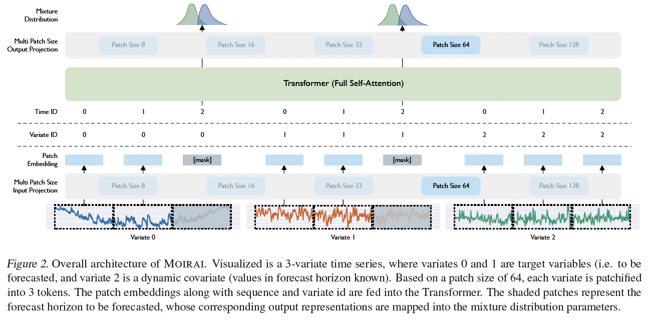
Framework

• (non-overlapping) patch-based approach
• masked encoder architecture

Proposed modifications

• “flatten” MTS: to extend the architecture to the any-variate setting
  • consider all variates as a single sequence

Input projection

• projected into vector representations via a multi patch size input projection layer

[mask]

• learnable embedding
• replaces patches falling within the forecast horizon

Output projection

• output tokens are then decoded via the multi patch size output projection into the parameters of the mixture distribution.

Etc

• (non-learnable) instance normalization (Kim et al., 2022)
• encoder-only Transformer architecture
  • use pre-normalization (Xiong et al., 2020)
  • replace all LayerNorms with RMSNorm (Zhang & Sennrich, 2019),
  • query-key normalization (Henry et al., 2020)
• non-linearity in FFN layers: SwiGLU (Shazeer, 2020)

a) Multi Patch Size Projection Layers

Single model should possess the capability to handle TS spanning a wide range of frequencies

If single patch size?

• one-model-per-dataset paradigm :(

Flexible strategy:

• “Larger” patch size to handle high-frequency data
  • thereby lower the burden of the quadratic computation cost of attention while maintaining a long context length.
• “Smaller” patch size for low-frequency data
  • to transfer computation to the Transformer layers, rather than relying solely on simple linear embedding layers. To implement

\(\rightarrow\) Propose learning “multiple” input and output embedding layers

• each associated with varying patch sizes

• only learn one set of projection weights per patch size

  • which is shared amongst frequencies if there is an overlap based on the settings.

b) Any-Variate Attention

Universal forecasters: must be equipped to handle arbitrary MTS

Existing TS Transformers (often)

• rely on an independent variate assumption
• limited to a single dimensionality due to embedding layers mapping \(\mathbb{R}^{d_y} \rightarrow \mathbb{R}^{d_h}\),

Solution) By flattening a MTS to consider all variates as a single sequence

• Requires variate encodings
  • to enable the model to disambiguate between different variates
• Need to ensure that …
  • permutation equivariance w.r.t. variate ordering
  • permutation invariance w.r.t. variate indices

Propose Any-variate Attention

\(\rightarrow\) Leverage binary attention biases to encode variate indices.

Attention score \(A_{i j, m n} \in \mathbb{R}\)

• btw the \((i, m)\)-th query & and \((j, n)\)-th key
  • \(i\) : time index
  • \(m\) : variate index
• \(A_{i j, m n}= \frac{\exp \left\{E_{i j, m n}\right\}}{\sum_{k, o} \exp \left\{E_{i k, m o}\right\}}\).
  • \(E_{i j, m n}= \left(\boldsymbol{W}^Q \boldsymbol{x}_{i, m}\right)^T \boldsymbol{R}_{i-j}\left(\boldsymbol{W}^K \boldsymbol{x}_{j, n}\right) +u^{(1)} * \mathbb{1}_{\{m=n\}}+u^{(2)} * \mathbb{1}_{\{m \neq n\}}\).
  • \(\boldsymbol{W}^Q \boldsymbol{x}_{i, m} \in \mathbb{R}^{d_h}\): query vectors
  • \(\boldsymbol{W}^K \boldsymbol{x}_{j, n} \in \mathbb{R}^{d_h}\): key vectors
  • \(\boldsymbol{R}_{i-j} \in \mathbb{R}^{d_h \times d_h}\) : rotary matrix ( \(\mathrm{Su}\) et al., 2024)
  • \(u^{(1)}, u^{(2)} \in \mathbb{R}\) : learnable scalars for each head in each layer,

Binary attention bias

• allows for disambiguation between variates via attention scores,

\(\rightarrow\) fulfills permutation equivariance/invariance w.r.t. variate ordering/indices

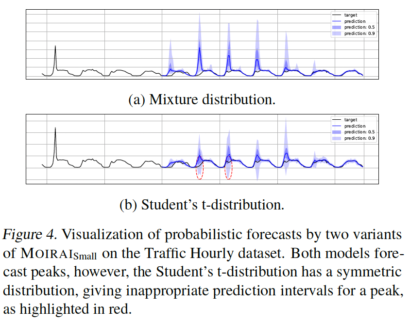
c) Mixture Distribution

Mixture of parametric distributions (of \(c\) components)

• \(p\left(\mathbf{Y}_{t: t+h} \mid \hat{\boldsymbol{\phi}}\right)=\sum_{i=1}^c w_i p_i\left(\mathbf{Y}_{t: t+h} \mid \hat{\phi}_i\right)\).
  • where \(\hat{\boldsymbol{\phi}}=\left\{w_1, \hat{\phi}_1, \ldots, w_c, \hat{\boldsymbol{\phi}}_c\right\}\),
    • \(p_i\) is the \(i\)-th component’s p.d.f

Mixture components

• (1) Student’s \(\mathrm{t}\)-distribution
  • robust option for general time series
• (2) Negative binomial distribution
  • for positive count data
• (3) Log-normal distribution
  • to model right-skewed data commonly across economic and and natural phenomena
• (4) Low variance normal distribution
  • for high confidence predictions.

(2) Unified Training

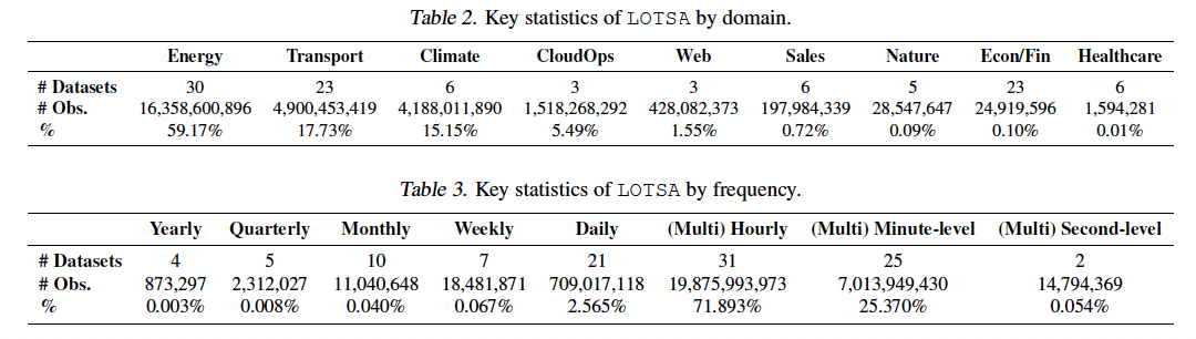
a) LOTSA data

Existing work: relied on three primary sources of data

• (1) Monash Time Series Forecasting Archive (Godahewa et al., 2021)
• (2) GluonTS library (Alexandrov et al., 2020)
• (3) Popular LTSF benchmark (Lai et al., 2018; Wu et al., 2021).
• (4) Das et al. (2023b)

(1) & (2): diverse domains, but constrained in size

• approximately 1B observations combined

  (\(\leftrightarrow\) LLMs are trained on trillions of tokens)

(4) Private dataset based on Google Trends

• but lacks diversity
• similarly sized at 1B observations

\(\rightarrow\) Tackle this issue head-on by building a large-scale archive of open TS datasets by collating publicly available sources of TS datasets.

\(\rightarrow\) Result: LOTSA

• 9 domains
• 27,646,462,733 observations

b) Pre-training

Optimize the mixture distribution log-likelihood

1) Data Distribution

• \[(\mathbf{Y}, \mathbf{Z}) \sim p(\mathcal{D})\]

• Defines how TS are sampled from the dataset

• Introduce the notion of sub-datasets

  \(p(\mathcal{D})=\) \(p(\mathbf{Y}, \mathbf{Z} \mid \mathbf{D}) p(\mathbf{D})\).

  • by decomposing the data distribution into a sub-dataset distribution
  • TS distribution conditioned on a sub-dataset

• Procedure

  • Step 1) Sample a sub-dataset from \(p(\mathbf{D})\)
  • Step 2) Given that sub-dataset, we sample a TS

Notation

• \(K\) sub-datasets of \(\boldsymbol{D}_k\)
  • represents the set of indices of TS belonging to sub-dataset \(k\)
• \(p\left(\boldsymbol{Y}^{(i)}, \boldsymbol{Z}^{(i)} \mid \boldsymbol{D}_k\right)=\frac{T_{i * 1}\left\{i \in \boldsymbol{D}_k\right\}}{\sum_{j \in \boldsymbol{D}_k} T_j}\),
  • proportionate to the number of observations

Due to data imbalance …

• avoid sampling sub-datasets proportionately
• instead cap the contribution of each sub-dataset at \(\epsilon=0.001\),

\(\rightarrow\) \(p\left(\boldsymbol{D}_k\right)=\frac{\omega_k}{\sum_{i=1}^K \omega_i}\)

• where \(\omega_k=\frac{\min \left( \mid \boldsymbol{D}_k \mid , \epsilon\right)}{\sum_i^K \mid \boldsymbol{D}_i \mid }\) and \(\mid \boldsymbol{D}_k \mid =\sum_{i \in \boldsymbol{D}_k} T_i\).

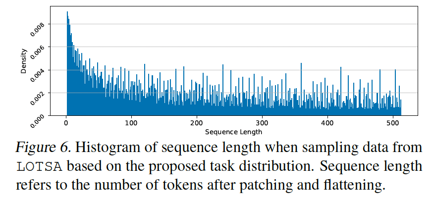
2) Task Distribution

• Fixed context and prediction length (X)
• Sample from a task distribution, \((\mathrm{t}, l, \mathrm{~h}) \sim p(\mathcal{T} \mid \mathcal{D})\)
• In practice, rather than sampling \(t, l, h\), given a TS,
  • Step 1) Crop a uniformly sampled window
    • whose length is uniformly sampled from a range (2,512)
  • Step 2) Split into lookback and horizon segments
    • prediction length is uniformly sampled as a proportion (within a range (0.15,0.5))
  • Step 3) Further augment training by
    • (1) Uniformly subsampling MTS in the variate dimension
    • (2) Constructing MTS from sub-datasets with univariate TS
      • by randomly concatenating them
• Etc) # of variates is sampled from a beta-binomial distribution
  • maximum of 128 variates, with mean \(\approx 37\)

3) Training

4. Experiments

(1) In-distribution Forecasting

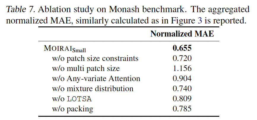
a) Monash benchmark

• aim to measure generalization capability across diverse domains.

• (Note that Monash \(\in\) LOTSA )

b) Train & Test

• only include the train set
• holding out the test set
  • use for in-distribution evaluation.

c) Setting

• context length of 1000

• patch size of 32 for all frequencies,

  ( except for quarterly data with a patch size of 8 )

d) Result

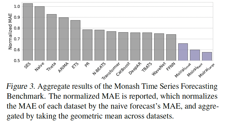
• Note that each baseline is typically trained individually per dataset or per TS within a dataset!!

  (\(\leftrightarrow\) MOIRAIA: single model)

(2) OOD / Zero-Shot Forecasting

a) Unseen target datasets

Most universal forecasters:

• currently do not yet have open weights avaiable for evaluation.

Problem of comparing zero-shot methods

• not having a standard held-out test split

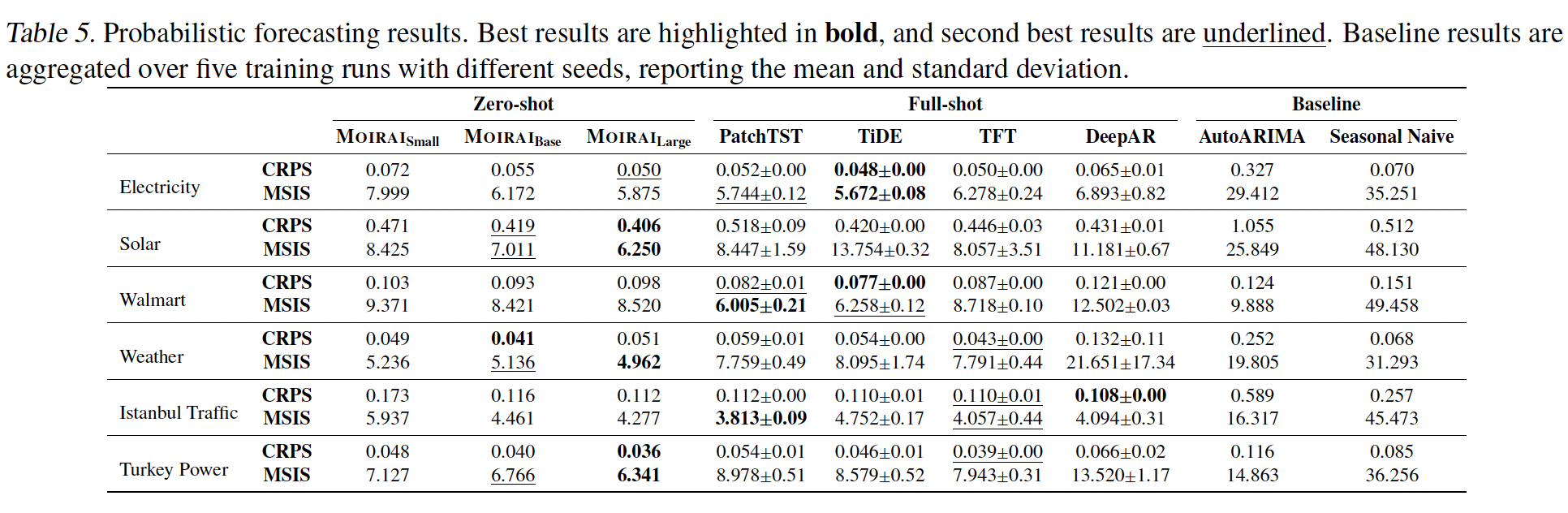
b) Probabilistic Forecasting

• Evaluate on seven datasets
• Rolling evaluation setup with stride equal to prediction length.
  • defined for each dataset based on frequency.

• Metric: CRPS & Mean Scaled Interval Score (MSIS)

• For each dataset and baseline, we perform hyperparameter tuning on a validation CRPS, and report results averaged over five training runs with different seeds.

For MOIRAI, perform…

• (1) Inference time tuning

• (2) Selecting

  • context length from {1000, 2000, 3000, 4000, 5000}
  • and patch sizes based on frequency

  on the validation CRPS.

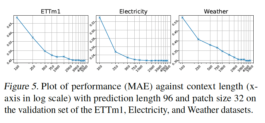
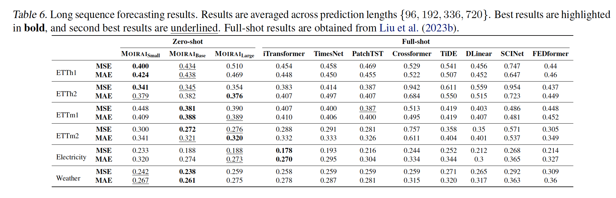
c) Long Sequence Forecasting

(3) Ablation Study