Parametric Augmentation for Time Series Contrastive Learning

Parametric Augmentation for Time Series Contrastive Learning

Contents

1. Abstract
2. Related Work
3. Methodology
   1. Notations
   2. What are the good views for CL?
   3. How to achieve good views?

Abstract

Constructing postive pair?

\(\rightarrow\) Impractical to visually inspect the temporal structures in TS ( + due to diversity in TS )

Proposal

• (1) Analyze TS data augmentation using information theory
• (2) Summarize most commonly adopted augmentations in a unified format
• (3) AutoTCL
  • CL with parametric augmentation
  • Adaptively employed to support TS representation learning
  • Encoder-agnostic
• (4) Experiments
  • Univariate forecasting tasks
  • classification

Code: https://github.com/AslanDing/AutoTCL.

1. Related work

(1) Adaptive Data Augmentation

Choice of optimal augmentation methods depends on the specific task and dataset

Adaptive selection of augmentation methods ( in the visual domain )

• ex) AutoAugment (Cubuk et al., 2019): RL to search for the best combination of policies.
• ex) CADDA (Rommel et al., 2022): Gradient-based class-wise method to support larger search spaces for EGG signals
• ex) DACL (Verma et al., 2021): Domain-agnostic approach that does not rely on domain-specific data augmentation techniques
• ex) MetAug (Li et al., 2022), Hallucinator (Wu et al., 2023): Augmentations in the latent space

InfoMin theory ( in CL framework )

• Guide the selection of good views for CL in the vision domain (Tian et al., 2020)
• Proposes a flow-based generative model to transfer images from natural color spaces into novel color spaces for data augmentation.

\(\rightarrow\) Limitation) Given the complexity of TS, directly applying the InfoMin framework may not be suitable.

(Proposal) AutoTCL

• End-to-end differentiable method
• Automatically learn the optimal augmentations for each TS instance.

2. Methodology

Questions.

• Q1) What are the good views for CL?
• Q2) How to obtain good views for each TS instance for CL?

(1) Notations

TS: \(T \times F\) matrix

Encoder: \(f\) ….. maps \(x\) from \(\mathbb{R}^{T \times F}\) to \(\mathbb{R}^D\)

(2) What are the good views for CL?

Good views preserve the semantics and provide sufficient variances

( SL )

• Semantics of an instance is usually approximated with the label

( SSL )

• Semantics-preserving is much less explored

• Semantics of …

  • CV & NLP: can be manually verified
  • TS: not easily recognizable to humans

  \(\rightarrow\) Challenging to apply strong yet faithful data augmentations!

To avoid the degenerate solutions … InfoMin utilizes an invertible flow-based function

• Flow-based function: \(g\)
  • Generate a view \(v\) for an input \(x\)
  • \(x\) can be restored by \(x=g^{-1}(v)\).
• However, from the information theory perspective …
  • Invertible functions fail to include extra variance to the original variable

[Property 1]

If view \(\mathrm{v}\) is generated from \(\mathrm{x}\) with an invertible function \(\mathrm{v}=g(\mathrm{x})\), then \(H(\mathrm{v})=H(\mathrm{x})=\) \(M I(\mathrm{x} ; \mathrm{v})\),

= Shows that the entropy of the augmented view, \(H(\mathrm{v})\), is no larger than that of original data, \(H(\mathrm{x})\)

= Existing DA don’t bring new information for input instances

= Limits their expressive power for TS CL

\(\rightarrow\) Solution: AutoTCL

AutoTCL

• Novel factorized augmentation technique
• Details
  • Given \(x\), assume that \(x\) can be factorized into two parts
    • (1) Informative \(x^*\)
    • (2) Task-irreverent part \(\Delta x\).
  • \(x=x^*+\Delta x\).
• Informative part \(x^*\)
  • encodes the semantics of the original \(x\).
• Define good views for CL as follows!

Definition 1 (Good View)

Given a random variable \(\mathrm{x}\) with its semantics \(\mathrm{x}^*\),

a good view \(\mathrm{v}\) for CL can be achieved by \(\mathrm{v}=\eta\left(g\left(\mathrm{x}^*\right), \Delta \mathrm{v}\right)\), where ..

• \(\mathrm{g}\) is an inverible function
• \(\Delta \mathrm{v}\) is a task-irrelevant noise
  • satisfying \(H(\Delta \mathrm{v}) \geq H(\Delta \mathrm{x})\)
• \(\eta\) is an augmentation function
  • that satisfies that \(g\left(\mathrm{x}^*\right) \rightarrow \mathrm{v}\) is a one-to-many mapping.

Good view

• maintains the useful information in the original variable
• includes a larger variance to boost the robustness of encoder training

Theoretically show that the defined good view has the following properties:

• Property 2 (Task Agnostic Label Preserving)
• Property 3 (Containing More Information)

Property 2 (Task Agnostic Label Preserving)

\(M I(\mathrm{v} ; \mathrm{y})=M I(\mathrm{x} ; \mathrm{y})\).

• If a variable \(\mathrm{v}\) is a good view of \(\mathrm{x}\), and the downstream task label \(y\) is independent to noise in \(\mathrm{x}\),

  the mutual information between \(\mathrm{v}\) and \(\mathrm{y}\) is equivalent to that between raw input \(\mathrm{x}\) and \(\mathrm{y}\),

Property 3 (Containing More Information)

\(H(\mathrm{v}) \geq H(\mathrm{x})\).

• A good view \(\mathrm{v}\) contains more information comparing to the raw input \(\mathrm{x}\)

+ Good view is flexible to the choice of \(\Delta \mathrm{v}\)

= Strong augmentations = incorporate more diversity for training.

(3) How to achieve good views?

Factorized augmentation

• to preserve task-agnostic labels
• to improve the diversity of views

Practical instantiation to obtain good views

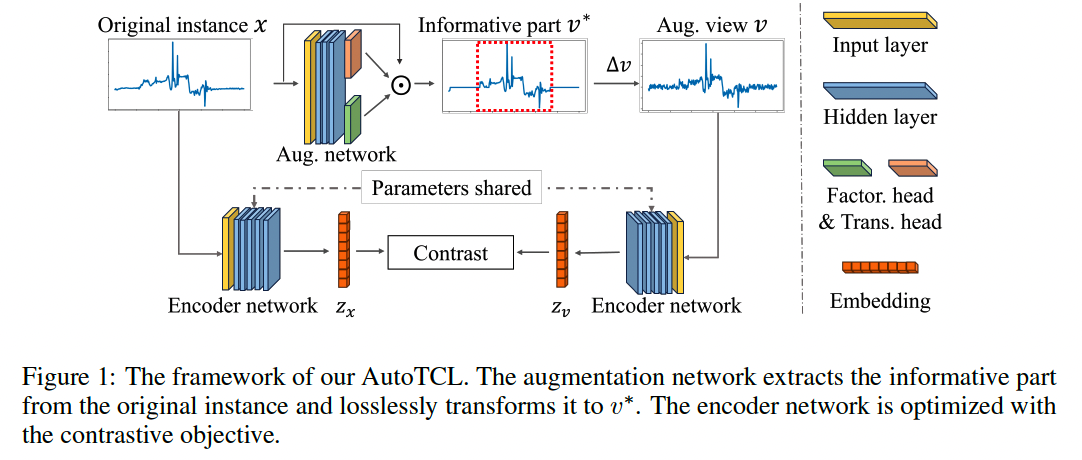
• based on parametric augmentations ( Fig 1 )

(1) Factorization function \(h: \mathbb{R}^{T \times F} \rightarrow\{0,1\}^{T \times 1}\)

• To discover where are the informative parts in input
• \(\boldsymbol{h}=h(x), \quad x^*=\boldsymbol{h} \odot x, \quad \Delta x=x-x^*\).
  • \(\boldsymbol{h}\) : Factorization mask
  • \(x^*\): Informative component
  • \(\Delta x\) : Noise component

Impractical to have a universal mask that applies to all TS instances

To ensure each instance has a suitable transform adaptively …

(2) Non-zero mask \(\boldsymbol{g} \in \mathbb{R}_{\neq 0}^T\)

• \(\boldsymbol{g}=g(x), \quad v^*=\boldsymbol{g} \odot x^*\).

• via Parametric mask generator: \(g: \mathbb{R}^{T \times F} \rightarrow \mathbb{R}_{\neq 0}^T\),

• Lossless, as the original \(x^*\) can be restored by \(x^*=\frac{1}{\boldsymbol{g}} \odot v^*\).

• Learn lossless transformation through a data-driven approach

Good view \(v\) can be represented as follows

\(v =\eta\left(v^*, \Delta v\right)=\eta\left(\boldsymbol{g} \odot x^*, \Delta v\right) =\eta(g(x) \odot h(x) \odot x, \Delta v)\).

• by integrating
  • the factorization function
  • the mask generator
• by introducing random noise for perturbation \((\Delta v)\).